User login
Hospital Testing Overuse Done to Reassure Patients, Families
Clinical Question: What is the extent of, and factors associated with, testing overuse in U.S. hospitals for pre-operative evaluation and syncope.
Background: Little is known about the extent and drivers of overuse by hospitalists.
Study design: Two vignettes (pre-operative evaluation and syncope) were mailed to hospitalists. They were asked to identify what most hospitalists at their institution would recommend and “the most likely primary driver of the hospitalist’s decision.”
Setting: Random selection of hospitalists from SHM member database and SHM national meeting attendees.
Synopsis: Investigators mailed 1,753 surveys and received a 68% response rate. For the pre-operative evaluation vignette, 52% of hospitalists reported overuse of pre-operative testing. When a family member was a physician and requested further testing, overuse increased significantly to 65%. For the syncope vignette, any choice involving admission was considered overuse.
Eighty-two percent of respondents reported overuse; when the wife was a lawyer or requested further testing, overuse remained the same. Overuse in both cases was more frequent due to a hospitalist’s desire to reassure patients or themselves, rather than a belief that it was clinically indicated (pre-operative evaluation, 63% vs. 37%; syncope, 69% vs. 31%, P<0.001).
The survey responses do not necessarily represent actual clinical choices, and the hospitalist sample may not be representative of all hospitalists; however, this study shows that efforts to reduce overuse in hospitals need to move beyond financial incentives and/or informing providers of evidence-based recommendations.
Bottom line: A survey of hospitalists showed substantial overuse in two common clinical situations, syncope and pre-operative evaluation, mostly driven by a desire to reassure patients, families, or themselves.
Citation: Kachalia A, Berg A, Fagerlin A, et al. Overuse of testing in preoperative evaluation and syncope: a survey of hospitalists. Ann Intern Med. 2015;162(2):100-108.
Functional Impairment Boosts Readmission for Medicare Seniors
Clinical question: Is functional impairment associated with an increased risk of 30-day readmission?
Background: Many Medicare seniors suffer from some level of impairment in functional status, which, in turn, has been linked to high healthcare utilization. Studies that examine the role of functional impairment with readmission rates are limited.
Study design: Prospective, cohort study.
Setting: Seniors enrolled in the Health and Retirement Study (HRS) with Medicare hospitalizations from Jan. 1, 2000, to Dec. 31, 2010.
Synopsis: The primary outcome was readmissions within 30 days of discharge. Activities of daily living (ADL) scale and instrumental ADL were used as measures of functional impairment.
Overall, 48.3% of patients had preadmission functional impairments with a readmission rate of 15.5%. There was a progressive increase in the adjusted risk of readmission as the degree of functional impairment increased: 13.5% with no functional impairment, 14.3% with difficulty in one or more instrumental ADLs (OR 1.06; 95% CI 0.94-1.20), 14.4% with difficulty in one or more ADLs (OR 1.08; 95% CI 0.96-1.21), 16.5% with dependency in one or two ADLs (OR, 1.26; 95% CI 1.11-1.44), and 18.2% with dependency in three or more ADLs (OR 1.42; 95% CI 1.20-1.69).
This observation was more pronounced in patients admitted for heart failure, MI, and pneumonia (16.9% readmission rate for no impairment vs. 25.7% dependency in three or more ADLs, OR 1.70; 95% CI 1.04-2.78).
Although the study is limited by reliance on survey data and Medicare claim data, functional status may be an important variable in calculating readmission risk and a potential target for intervention.
Bottom line: Functional impairment is associated with an increased risk of 30-day readmission, especially in patients admitted for heart failure, MI, and pneumonia.
Citation: Greysen SR, Stijacic Cenzer I, Auerbach AD, Covinsky KE. Functional impairment and hospital readmission in Medicare seniors. JAMA Intern Med. 2015;175(4):559-565.
Delirium, Falls Reduced by Nonpharmacological Intervention
Clinical question: Are multicomponent, nonpharmacological interventions effective in decreasing delirium and falls?
Background: Delirium is prevalent among elderly hospitalized patients and is associated with increased morbidity, length of stay, healthcare costs, and risk of institutionalization. Multicomponent nonpharmacologic interventions have been used to prevent incident delirium in the elderly, but data regarding their effectiveness and impact on preventing poor outcomes are lacking.
Study design: Systematic literature review and meta-analysis.
Setting: Review of medical databases from Jan. 1, 1999, to Dec. 31, 2013.
Synopsis: Fourteen studies were included involving 4,267 elderly patients from 12 acute medical and surgical sites from around the world. There was a 53% reduction in delirium incidence associated with multicomponent, nonpharmacological interventions (OR, 0.47; 95% CI, 0.38-0.58). The odds of falling were 62% lower among intervention patients compared with controls (2.79 vs. 7.05 falls per 1,000 patient-days). The intervention group also showed a decrease in length of stay, with a mean difference of -0.16 (95% CI, -0.97 to 0.64) days and a 5% lower chance of institutionalization (95% CI, 0.71 to 1.26); however, the differences were not statistically significant.
Although the small number and heterogeneity of the studies included limited the analysis, the use of nonpharmacologic interventions appears to be a low-risk, low-cost strategy to prevent delirium. The challenge for the hospitalist in developing a nonpharmacological protocol is to determine which interventions to include; the study did not look at which interventions were most effective.
Bottom line: The use of multicomponent nonpharmacological interventions in older patients can lower the risk of delirium and falls.
Citation: Hshieh TT, Yue J, Oh E, et al. Effectiveness of multicomponent nonpharmacological delirium interventions: a meta-analysis. JAMA Intern Med. 2015;175(4):512-520.
Bridging Anticoagulation for Patients with Atrial Fibrillation
Clinical question: Is bridging anticoagulation for procedures associated with a higher bleeding risk and increased adverse outcomes compared to no bridging?
Background: Practice guidelines have been published to determine when, how, and on whom to bridge anticoagulation for procedures; however, uncertainty remains as to whether or not bridging changes outcomes.
Study design: Prospective, observational study.
Setting: Outcomes Registry for Better Informed treatment of Atrial Fibrillation (ORBIT-AF) study.
Synopsis: Investigators included 10,132 patients who were 18 years and older, with a baseline EKG documenting atrial fibrillation (Afib) and undergoing procedures. Interruptions of oral anticoagulation for a procedure, as well as the use and type of bridging method, were recorded. Six hundred sixty-five patients (24%) used bridging anticoagulation (73% low molecular weight heparin, 15% unfractionated heparin) prior to a procedure. Bridged patients were more likely to have had a mechanical valve replacement (9.6% vs. 2.4%, P<0.0001) and prior stroke (22% vs. 15%, P=0.0003).
Multivariate adjusted analysis showed that bridged patients, compared with non-bridged patients, had higher rates of bleeding (5.0% vs. 1.3%, adjusted odds ratio (OR) 3.84, P<0.0001) and an increased risk for adverse events, including the composite of myocardial infarction (MI), bleeding, stroke or systemic embolism, hospitalization, or death within 30 days (OR 1.94, 95% CI 1.38-271, P=0.0001). Rates of CHADS2 ≥2 or CHA2DS2-VASc score ≥2 were similar between bridged and nonbridged patients.
These results are observational and, therefore, a causal relationship cannot be established; however, the Effectiveness of Bridging Anticoagulation for Surgery (BRIDGE) study will give us more insight and answers.
Bottom line: Bridging anticoagulation prior to procedures is associated with a higher risk of bleeding and adverse outcomes.
Citation: Steinberg BA, Peterson ED, Kim S, et al. Use and outcomes associated with bridging during anticoagulation interruptions in patients with atrial fibrillation: Findings from the Outcomes Registry for Better Informed Treatment of Atrial Fibrillation (ORBIT-AF). Circulation. 2015;131(5):488-494.
Family Medicine’s Increasing Presence in Hospital Medicine
Years ago, I struggled with a difficult decision. Given the fact that the military disallowed dual training tracks, such as internal medicine/pediatrics (med/peds), I had to choose from internal medicine (IM), pediatrics (Peds), or family practice (FP) residencies. My personal history and experiential data remained incomplete and the view ahead blurry; still, the choice remained.
Over time, I’ve embraced the uncertainty inherent in most analyses. Such is the case with the current composition of specialties that make up hospital medicine nationwide. Available data remains in flux, yet I see apparent trends.
A new question in the 2014 State of Hospital Medicine (SOHM) report asked, “Did your hospital medicine group employ hospitalist physicians trained and certified in the following specialties…?” Strikingly, a full 59% of groups serving adult patients only reported having at least one family medicine-trained provider in their midst! And in these adult-only practices, 98% of groups utilized at least one internal medicine physician, 24% reported a med/peds doc, and none reported pediatricians.

Meanwhile, of 40 groups caring for children only, 95% reported using pediatrics, 2.5% internal medicine (huh?), 22.5% med/peds, and zero FPs. The 19 groups serving both adults and children revealed participation from all four nonsurgical hospitalist specialties (IM, peds, FP, med/peds).
So what is the specialty distribution of medical hospitalists overall? There’s no good data about this.
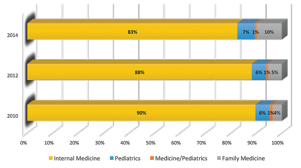
The 2014 Medical Group Management Association (MGMA) sample, licensed for use in SOHM, reported data for roughly 4,200 community hospital medicine providers: 82% were internal medicine, 10% family medicine, 7% pediatrics, and <1% med/peds. MGMA, however, cautions against assuming that this represents the entire population of hospitalists and their training. Although representative of the groups who participated in the survey, it may not be representative of groups that didn’t participate, and thus it would be misleading to suggest that this distribution holds true nationally.
In an effort to corroborate the MGMA distribution, I reviewed other compensation and productivity surveys; one such survey, conducted by the American Medical Group Association, reported hospitalists by training program. It contained over 3,700 community hospital providers—89% internal medicine, 6% family medicine, 5% pediatrics—but did not inquire about medicine/pediatrics.
Finally, if one combines the academic and community provider samples from MGMA (n=4,867), the distribution is 80% IM, 8.5% FP, 10% peds, and <1% med/peds.
Which of these, if any, is the actual distribution of nonprocedural hospitalists? Although we cannot know exactly, I believe something close to the following to be current state: internal medicine 80%, family medicine 10%, pediatrics 10%, and medicine/pediatrics <1%.
It is clear from survey trends that the proportion of family medicine providers is growing, while the internal medicine super-majority is shrinking somewhat. Pediatrics appears to remain stable as a proportion of the total, as does med/peds, with the latter unable to grow in numbers proportionally given the small number of providers nationally compared to the other three fields.
The growth of family medicine-trained hospitalists relates to the continued high demand for the profession, with such residents comprising the largest pool of available providers, second only to internal medicine.
Based on the SHM survey, family medicine hospitalists seem to practice similarly to IM; they generally see adults only. It appears that they are accepted into traditional adult hospitalist practices, readily contrasting with groups serving children, which report no FP participation. Meanwhile, med/peds hospitalists provide care across the spectrum of hospitalist groups, though they often report splitting their duties between adults-only services and pediatric services.
As for me, a generation removed from my election of a family practice internship and subsequent transition to internal medicine residency, I should not have worried so. Both paths can lead to hospital medicine.
Dr. Ahlstrom is a hospitalist at Indigo Health Partners in Traverse City, Mich., and a member of SHM’s Practice Analysis Committee.
Years ago, I struggled with a difficult decision. Given the fact that the military disallowed dual training tracks, such as internal medicine/pediatrics (med/peds), I had to choose from internal medicine (IM), pediatrics (Peds), or family practice (FP) residencies. My personal history and experiential data remained incomplete and the view ahead blurry; still, the choice remained.
Over time, I’ve embraced the uncertainty inherent in most analyses. Such is the case with the current composition of specialties that make up hospital medicine nationwide. Available data remains in flux, yet I see apparent trends.
A new question in the 2014 State of Hospital Medicine (SOHM) report asked, “Did your hospital medicine group employ hospitalist physicians trained and certified in the following specialties…?” Strikingly, a full 59% of groups serving adult patients only reported having at least one family medicine-trained provider in their midst! And in these adult-only practices, 98% of groups utilized at least one internal medicine physician, 24% reported a med/peds doc, and none reported pediatricians.
Meanwhile, of 40 groups caring for children only, 95% reported using pediatrics, 2.5% internal medicine (huh?), 22.5% med/peds, and zero FPs. The 19 groups serving both adults and children revealed participation from all four nonsurgical hospitalist specialties (IM, peds, FP, med/peds).
So what is the specialty distribution of medical hospitalists overall? There’s no good data about this.
The 2014 Medical Group Management Association (MGMA) sample, licensed for use in SOHM, reported data for roughly 4,200 community hospital medicine providers: 82% were internal medicine, 10% family medicine, 7% pediatrics, and <1% med/peds. MGMA, however, cautions against assuming that this represents the entire population of hospitalists and their training. Although representative of the groups who participated in the survey, it may not be representative of groups that didn’t participate, and thus it would be misleading to suggest that this distribution holds true nationally.
In an effort to corroborate the MGMA distribution, I reviewed other compensation and productivity surveys; one such survey, conducted by the American Medical Group Association, reported hospitalists by training program. It contained over 3,700 community hospital providers—89% internal medicine, 6% family medicine, 5% pediatrics—but did not inquire about medicine/pediatrics.
Finally, if one combines the academic and community provider samples from MGMA (n=4,867), the distribution is 80% IM, 8.5% FP, 10% peds, and <1% med/peds.
Which of these, if any, is the actual distribution of nonprocedural hospitalists? Although we cannot know exactly, I believe something close to the following to be current state: internal medicine 80%, family medicine 10%, pediatrics 10%, and medicine/pediatrics <1%.
It is clear from survey trends that the proportion of family medicine providers is growing, while the internal medicine super-majority is shrinking somewhat. Pediatrics appears to remain stable as a proportion of the total, as does med/peds, with the latter unable to grow in numbers proportionally given the small number of providers nationally compared to the other three fields.
The growth of family medicine-trained hospitalists relates to the continued high demand for the profession, with such residents comprising the largest pool of available providers, second only to internal medicine.
Based on the SHM survey, family medicine hospitalists seem to practice similarly to IM; they generally see adults only. It appears that they are accepted into traditional adult hospitalist practices, readily contrasting with groups serving children, which report no FP participation. Meanwhile, med/peds hospitalists provide care across the spectrum of hospitalist groups, though they often report splitting their duties between adults-only services and pediatric services.
As for me, a generation removed from my election of a family practice internship and subsequent transition to internal medicine residency, I should not have worried so. Both paths can lead to hospital medicine.
Dr. Ahlstrom is a hospitalist at Indigo Health Partners in Traverse City, Mich., and a member of SHM’s Practice Analysis Committee.
Society of Hospital Medicine Names 2015 Excellence Award Winners
OUTSTANDING SERVICE IN HOSPITAL MEDICINE

Dr. Sheehy has been a national role model for how SHM and its members can work together to achieve positive change in healthcare both in research and health policy. As a result of her published research on the “two-midnight rule” and observation status, Dr. Sheehy and SHM were invited to testify before the House Committee on Ways and Means Subcommittee on Health and the Senate Special Committee on Aging. In both of these instances, Dr. Sheehy shared the honor, bringing all of hospital medicine into the spotlight as a field of experts in this area.
EXCELLENCE IN RESEARCH

Dr. Brotman’s research has helped improve the care of thousands—if not millions—of hospitalized patients. He has achieved a prolific research portfolio while actively practicing as a hospitalist, as well as director of the hospitalist service at Johns Hopkins Hospital in Baltimore. His research has focused on VTE and patient education and communication. He has published more than 60 papers, multiple invited review articles, and a number of editorials. Since 1999, his research efforts have resulted in funding of more than $21 million.
CLINICAL EXCELLENCE

Dr. Kim has established one of the largest surgical consult and co-management services in the country, from the ground up, at an institution where many surgeons historically did not trust employed hospitalists. The success of the consult service required a total reorientation of institutional attitudes and culture, a feat Dr. Kim was able to achieve by providing superlative medical care to patients on nonmedical services. Dr. Kim is now nationally recognized as a leader in inpatient hospital care and a critical part of the neurosurgery team at Rush University Medical Center in Chicago.
EXCELLENCE IN TEACHING

Dr. Feldman founded new Urban Health residency training programs at Johns Hopkins. The medicine-pediatrics residency program and internal medicine primary care track admitted their first group of interns in July 2010 and 2011, respectively, and graduated those first cohorts last June. This medicine-pediatrics program is the first and only one of its kind in the nation. Dr. Feldman secured over $6 million in federal and foundation grant funding to support this endeavor.
At the same time, he led a team effort to build a perioperative and consultative medicine curriculum now known as “Consultative and Perioperative Medicine Essentials for Hospitalists,” which can be found at SHMconsults.com. With more than 18,000 users learning from more than 30 modules, this curriculum is now SHM’s flagship CME offering and a key resource for those preparing for the Focused Practice in Hospital Medicine exam. The curriculum has been built with over $1 million in industry grant funding.
EXCELLENCE IN HOSPITAL MEDICINE FOR NONPHYSICIANS

Cardin is deeply committed to collaborating with physicians on the integration of the role of NPs and PAs in hospital medicine, and in building a sense of community among NPs and PAs who are working in hospital medicine. She has worked toward these goals locally, regionally, and nationally through her participation and leadership in SHM.
As co-chair of the Quality Improvement Committee in the Section of Hospital Medicine at the University of Chicago, she has played a pivotal role in developing quality initiatives that directly benefit both her patients and providers in the section, including developing 360-degree evaluation tools and working on interdisciplinary projects, such as one that will enhance in-hospital glucose management. As an active member of the section’s Clinical Operations Committee, her input on ways to increase clinical efficiency, restructure services, and improve teamwork have led to improvements in the daily operations of her section.
At SHM, Tracy has provided leadership to NPs and PAs in her role as chair of the SHM NP-PA Committee. She is a core contributor to The Hospital Leader, SHM’s official blog, and was HM14 course director for the pre-course on the role of NPs and PAs in hospital medicine. This year, she was the first nonphysician to be nominated for the SHM board of directors.
EXCELLENCE IN HUMANITARIAN SERVICE

“Global Health Core,” organized by Phuoc Le, MD, MPH, has an established, clear agenda for clinical work, humanitarian aid, quality improvement, education, research, and fundraising. The group quickly grew from five to 12 faculty and brought focus to international efforts, with much of the work aimed at improving care at a particular hospital in Hinche (pronounced “Ench”), Haiti. Dr. Le and his team visit there, as well as other sites in Burundi and Liberia, several times a year, often taking residents and students as part of the University of California San Francisco’s Global Health Hospital Medicine Fellowship program. “Global Health Core” brought in supplies and medications after the 2010 earthquake and established a meaningful quality improvement program. They developed educational programs for trainees and created tighter partnerships with Partners in Health, and have begun to grow collaborations with several other university programs across the world.
Most recently, “Global Health Core” traveled to western Africa to care for patients inflicted with the Ebola virus, risking their lives for the care of the most vulnerable.
TEAM AWARD IN QUALITY IMPROVEMENT

Centripital, under the leadership of Jason Stein, MD, SFHM, is responsible for helping more than 50 hospital units around the world replicate the Accountable Care Unit (ACU) model of care. Dr. Stein is the inventor of the ACU and structured interdisciplinary bedside rounds, the author of an Accountable Care Unit implementation guide, and developer of the Structured Interdisciplinary Bedside Rounds certification program.
Centripital is a 501(c)(3) nonprofit based in Atlanta with the mission to train hospital professionals to work together in high-functioning, patient-centered teams. Centripital has helped more than 50 hospital units in 14 U.S. states and Australia replicate the ACU model by combining on-site educational sessions with mentored implementation. ACUs in the U.S. and Australia have been associated with improvements in a range of outcomes, including reduced in-hospital mortality, complications of care, length of stay, and average cost per case, along with increases in teamwork scores and patient satisfaction.
JUNIOR INVESTIGATOR AWARD

SHM’s Research Committee introduced a new award this year to recognize early-career hospitalist researchers who are leading the way in their field. Dr. Greysen is assistant professor at the UCSF School of Medicine and a hospitalist with training in social sciences and health outcomes research. His research focuses on transitions of care for hospitalized older adults and interventions to improve outcomes post-discharge. He is an active member in SHM’s research initiatives and associate editor for the Journal of Hospital Medicine.
OUTSTANDING SERVICE IN HOSPITAL MEDICINE
Dr. Sheehy has been a national role model for how SHM and its members can work together to achieve positive change in healthcare both in research and health policy. As a result of her published research on the “two-midnight rule” and observation status, Dr. Sheehy and SHM were invited to testify before the House Committee on Ways and Means Subcommittee on Health and the Senate Special Committee on Aging. In both of these instances, Dr. Sheehy shared the honor, bringing all of hospital medicine into the spotlight as a field of experts in this area.
EXCELLENCE IN RESEARCH
Dr. Brotman’s research has helped improve the care of thousands—if not millions—of hospitalized patients. He has achieved a prolific research portfolio while actively practicing as a hospitalist, as well as director of the hospitalist service at Johns Hopkins Hospital in Baltimore. His research has focused on VTE and patient education and communication. He has published more than 60 papers, multiple invited review articles, and a number of editorials. Since 1999, his research efforts have resulted in funding of more than $21 million.
CLINICAL EXCELLENCE
Dr. Kim has established one of the largest surgical consult and co-management services in the country, from the ground up, at an institution where many surgeons historically did not trust employed hospitalists. The success of the consult service required a total reorientation of institutional attitudes and culture, a feat Dr. Kim was able to achieve by providing superlative medical care to patients on nonmedical services. Dr. Kim is now nationally recognized as a leader in inpatient hospital care and a critical part of the neurosurgery team at Rush University Medical Center in Chicago.
EXCELLENCE IN TEACHING
Dr. Feldman founded new Urban Health residency training programs at Johns Hopkins. The medicine-pediatrics residency program and internal medicine primary care track admitted their first group of interns in July 2010 and 2011, respectively, and graduated those first cohorts last June. This medicine-pediatrics program is the first and only one of its kind in the nation. Dr. Feldman secured over $6 million in federal and foundation grant funding to support this endeavor.
At the same time, he led a team effort to build a perioperative and consultative medicine curriculum now known as “Consultative and Perioperative Medicine Essentials for Hospitalists,” which can be found at SHMconsults.com. With more than 18,000 users learning from more than 30 modules, this curriculum is now SHM’s flagship CME offering and a key resource for those preparing for the Focused Practice in Hospital Medicine exam. The curriculum has been built with over $1 million in industry grant funding.
EXCELLENCE IN HOSPITAL MEDICINE FOR NONPHYSICIANS
Cardin is deeply committed to collaborating with physicians on the integration of the role of NPs and PAs in hospital medicine, and in building a sense of community among NPs and PAs who are working in hospital medicine. She has worked toward these goals locally, regionally, and nationally through her participation and leadership in SHM.
As co-chair of the Quality Improvement Committee in the Section of Hospital Medicine at the University of Chicago, she has played a pivotal role in developing quality initiatives that directly benefit both her patients and providers in the section, including developing 360-degree evaluation tools and working on interdisciplinary projects, such as one that will enhance in-hospital glucose management. As an active member of the section’s Clinical Operations Committee, her input on ways to increase clinical efficiency, restructure services, and improve teamwork have led to improvements in the daily operations of her section.
At SHM, Tracy has provided leadership to NPs and PAs in her role as chair of the SHM NP-PA Committee. She is a core contributor to The Hospital Leader, SHM’s official blog, and was HM14 course director for the pre-course on the role of NPs and PAs in hospital medicine. This year, she was the first nonphysician to be nominated for the SHM board of directors.
EXCELLENCE IN HUMANITARIAN SERVICE
“Global Health Core,” organized by Phuoc Le, MD, MPH, has an established, clear agenda for clinical work, humanitarian aid, quality improvement, education, research, and fundraising. The group quickly grew from five to 12 faculty and brought focus to international efforts, with much of the work aimed at improving care at a particular hospital in Hinche (pronounced “Ench”), Haiti. Dr. Le and his team visit there, as well as other sites in Burundi and Liberia, several times a year, often taking residents and students as part of the University of California San Francisco’s Global Health Hospital Medicine Fellowship program. “Global Health Core” brought in supplies and medications after the 2010 earthquake and established a meaningful quality improvement program. They developed educational programs for trainees and created tighter partnerships with Partners in Health, and have begun to grow collaborations with several other university programs across the world.
Most recently, “Global Health Core” traveled to western Africa to care for patients inflicted with the Ebola virus, risking their lives for the care of the most vulnerable.
TEAM AWARD IN QUALITY IMPROVEMENT
Centripital, under the leadership of Jason Stein, MD, SFHM, is responsible for helping more than 50 hospital units around the world replicate the Accountable Care Unit (ACU) model of care. Dr. Stein is the inventor of the ACU and structured interdisciplinary bedside rounds, the author of an Accountable Care Unit implementation guide, and developer of the Structured Interdisciplinary Bedside Rounds certification program.
Centripital is a 501(c)(3) nonprofit based in Atlanta with the mission to train hospital professionals to work together in high-functioning, patient-centered teams. Centripital has helped more than 50 hospital units in 14 U.S. states and Australia replicate the ACU model by combining on-site educational sessions with mentored implementation. ACUs in the U.S. and Australia have been associated with improvements in a range of outcomes, including reduced in-hospital mortality, complications of care, length of stay, and average cost per case, along with increases in teamwork scores and patient satisfaction.
JUNIOR INVESTIGATOR AWARD
SHM’s Research Committee introduced a new award this year to recognize early-career hospitalist researchers who are leading the way in their field. Dr. Greysen is assistant professor at the UCSF School of Medicine and a hospitalist with training in social sciences and health outcomes research. His research focuses on transitions of care for hospitalized older adults and interventions to improve outcomes post-discharge. He is an active member in SHM’s research initiatives and associate editor for the Journal of Hospital Medicine.
Team Hospitalist Seats Seven New Members
Elizabeth A. Cook, MD

Dr. Cook has served as a hospitalist since 2001 and is medical director of the hospitalist division for Medical Associates of Central Virginia in Lynchburg, Va., where she provides management and coordination of care for acutely ill medical and surgical patients. She also serves as supervising physician at Matrix Medical Network, where she provides oversight to nurse practitioners through monthly chart reviews. Dr. Cook completed her medical degree at Vanderbilt University in Nashville and her internship at the University of North Carolina at Chapel Hill. Dr. Cook is board certified by the American Board of Family Medicine, is an SHM member, and serves on SHM’s Family Medicine Committee.
QUOTABLE: “I started as a hospitalist thinking it would be a transition to outpatient practice; however, I fell in love with the energy and experiences in the hospital. Being able to work closely with specialists, nursing, and other ancillary personnel to care for patients when they are most in need is both an opportunity and a privilege. I have moved into a leadership role, as well as returned to school for a masters in public health. I am excited about bringing my experience, passion, and interests to a role on the editorial board. I am also looking forward to working with other hospitalists outside my local area to move forward the practice of hospital medicine.”
Lisa Courtney, MBA, MSHA

Courtney serves as director of operations at Baptist Health Systems in Birmingham, Ala. She is responsible for accounts receivable management across a multi-hospital hospitalist program; develops, maintains, and attains budget objectives; and works with the medical directors and hospital staff on quality initiatives and process improvement opportunities.
QUOTABLE: “The hospitalist director position wasn’t a role I sought but one that I’m glad I accepted. My boss told me, ‘Hospitalist medicine is fun.’ It has taken a few years to stabilize staffing, but now I finally agree, hospitalist medicine is fun. … Hospitalists are an integral part of any healthcare system. They are vital in leading change and innovation to provide better care at lower cost. I feel blessed to be part of the team. As a new member of The Hospitalist’s editorial board, I hope to bring new ideas and topics to a broad audience while gaining the experience of working with some of the top physicians and administrative staff in their field.”
Joshua LaBrin, MD, SFHM

Dr. LaBrin is assistant clinical professor of internal medicine at the University of Utah at Salt Lake City. He also is a reviewer for Medical Education, Journal of Hospital Medicine, and Hospital Pediatrics. He completed his medical degree at Temple University in Philadelphia, Pa., and then his internship and residency at the University of Pittsburgh. He served as an HM fellow at Mayo Clinic in Rochester, Minn.
QUOTABLE: “Being a hospitalist made sense for me. I enjoy the intensive part of caring for the hospitalized setting in a team-based model. The dynamic nature of the hospital and the trainees never gets old. My mentors provided a glimpse of the impact and satisfaction I too could be a part of in hospital medicine.
James W. Levy, PA-C, SFHM

Levy serves as co-owner and vice president of human resources at iNDIGO Health Partners in Traverse City, Mich. He graduated from Indiana University in Bloomington and completed his PA training at Indiana University School of Medicine in Fort Wayne. He’d previously received certificates in emergency medical technology and operating room technology. He worked as a hospitalist from 1998 to 2013 and is a member of SHM’s NP/PA Committee.
QUOTABLE: “I believe the advent of hospitalist medicine is the single most important innovation I have seen in 40 years of patient care. Of the many rewards it has brought me, helping to assemble highly functioning hospitalist teams is the greatest. As a member of The Hospitalist’s editorial board, I hope to advance the cause of hospitalist medicine, in general, and especially as a way of benefitting small outlying hospitals and the patients they serve.”
Amanda T. Trask, MBA, MHA, SFHM

Trask is vice president for the national hospital medicine service line at Catholic Health Initiatives (CHI), a nonprofit, faith-based system operating in 19 states. Trask focuses on improving clinical and business outcomes through enhancing collaboration, improving processes, and optimizing current practices of hospitalist providers practicing in CHI hospitals. She earned her degrees at Georgia State University in Atlanta, where she was awarded the Public Health Service DHHS Traineeship Grant and several academic scholarships.
QUOTABLE: “Hospitalists have the opportunity to transform the delivery of acute care and beyond, as population health care models continue to advance. Being an administrative hospitalist leader allows me to be influential and involved in this transformation.
David Weidig, MD

Dr. Weidig is system director of hospital medicine for Aurora Health Care in Wisconsin. In 2007, he started the Aurora Hospital Medicine System with one program and six physicians; it has grown to 13 programs and over 150 FTEs. He is responsible for the co-development of the unit-based, RN-physician collaborative care model, recognized by the Robert Wood Johnson Foundation as a top intra-collaborative care model. Dr. Weidig completed his medical degree at Northwestern University in Chicago and his internal medicine residency at Scripps Mercy Hospital in San Diego. He served as president of SHM’s Pacific Northwest Chapter from 2005 to 2007 and is a member of the Multi-Site Hospitalist Leader Task Force.
QUOTABLE: “HM focuses on care delivery process improvement that has a dramatic effect both in efficiency and quality of outcomes. These improvements are reaching a scale that may be unprecedented in the history of U.S. healthcare. As a member of The Hospitalist’s editorial board, I hope to share ideas and work with others to further develop these care delivery models and enhance their effect.”
Robert Zipper, MD, MMM, SFHM

Dr. Zipper is a regional chief medical officer at Tacoma, Wash.-based Sound Physicians, where he provides operational oversight of Sound’s hospitalist, LTACH, post acute, and transitional care programs. He earned his master’s degree in medical management at Carnegie Mellon University in Pittsburgh, and his doctorate of medicine at Wayne State University in Detroit. He completed his internal medicine residency at Allegheny General Hospital in Pittsburgh. An active SHM member, he has served as chairman of the SHM Leadership Committee.
QUOTABLE: “My choice [to become a hospitalist] was more practical than anything else. I knew that I liked inpatient medicine, and I could not keep doing both inpatient and outpatient in the manner I was. I was forced to choose, and within a week of starting a focus on only hospital medicine, I knew it was the right one.”
Elizabeth A. Cook, MD
Dr. Cook has served as a hospitalist since 2001 and is medical director of the hospitalist division for Medical Associates of Central Virginia in Lynchburg, Va., where she provides management and coordination of care for acutely ill medical and surgical patients. She also serves as supervising physician at Matrix Medical Network, where she provides oversight to nurse practitioners through monthly chart reviews. Dr. Cook completed her medical degree at Vanderbilt University in Nashville and her internship at the University of North Carolina at Chapel Hill. Dr. Cook is board certified by the American Board of Family Medicine, is an SHM member, and serves on SHM’s Family Medicine Committee.
QUOTABLE: “I started as a hospitalist thinking it would be a transition to outpatient practice; however, I fell in love with the energy and experiences in the hospital. Being able to work closely with specialists, nursing, and other ancillary personnel to care for patients when they are most in need is both an opportunity and a privilege. I have moved into a leadership role, as well as returned to school for a masters in public health. I am excited about bringing my experience, passion, and interests to a role on the editorial board. I am also looking forward to working with other hospitalists outside my local area to move forward the practice of hospital medicine.”
Lisa Courtney, MBA, MSHA
Courtney serves as director of operations at Baptist Health Systems in Birmingham, Ala. She is responsible for accounts receivable management across a multi-hospital hospitalist program; develops, maintains, and attains budget objectives; and works with the medical directors and hospital staff on quality initiatives and process improvement opportunities.
QUOTABLE: “The hospitalist director position wasn’t a role I sought but one that I’m glad I accepted. My boss told me, ‘Hospitalist medicine is fun.’ It has taken a few years to stabilize staffing, but now I finally agree, hospitalist medicine is fun. … Hospitalists are an integral part of any healthcare system. They are vital in leading change and innovation to provide better care at lower cost. I feel blessed to be part of the team. As a new member of The Hospitalist’s editorial board, I hope to bring new ideas and topics to a broad audience while gaining the experience of working with some of the top physicians and administrative staff in their field.”
Joshua LaBrin, MD, SFHM
Dr. LaBrin is assistant clinical professor of internal medicine at the University of Utah at Salt Lake City. He also is a reviewer for Medical Education, Journal of Hospital Medicine, and Hospital Pediatrics. He completed his medical degree at Temple University in Philadelphia, Pa., and then his internship and residency at the University of Pittsburgh. He served as an HM fellow at Mayo Clinic in Rochester, Minn.
QUOTABLE: “Being a hospitalist made sense for me. I enjoy the intensive part of caring for the hospitalized setting in a team-based model. The dynamic nature of the hospital and the trainees never gets old. My mentors provided a glimpse of the impact and satisfaction I too could be a part of in hospital medicine.
James W. Levy, PA-C, SFHM
Levy serves as co-owner and vice president of human resources at iNDIGO Health Partners in Traverse City, Mich. He graduated from Indiana University in Bloomington and completed his PA training at Indiana University School of Medicine in Fort Wayne. He’d previously received certificates in emergency medical technology and operating room technology. He worked as a hospitalist from 1998 to 2013 and is a member of SHM’s NP/PA Committee.
QUOTABLE: “I believe the advent of hospitalist medicine is the single most important innovation I have seen in 40 years of patient care. Of the many rewards it has brought me, helping to assemble highly functioning hospitalist teams is the greatest. As a member of The Hospitalist’s editorial board, I hope to advance the cause of hospitalist medicine, in general, and especially as a way of benefitting small outlying hospitals and the patients they serve.”
Amanda T. Trask, MBA, MHA, SFHM
Trask is vice president for the national hospital medicine service line at Catholic Health Initiatives (CHI), a nonprofit, faith-based system operating in 19 states. Trask focuses on improving clinical and business outcomes through enhancing collaboration, improving processes, and optimizing current practices of hospitalist providers practicing in CHI hospitals. She earned her degrees at Georgia State University in Atlanta, where she was awarded the Public Health Service DHHS Traineeship Grant and several academic scholarships.
QUOTABLE: “Hospitalists have the opportunity to transform the delivery of acute care and beyond, as population health care models continue to advance. Being an administrative hospitalist leader allows me to be influential and involved in this transformation.
David Weidig, MD
Dr. Weidig is system director of hospital medicine for Aurora Health Care in Wisconsin. In 2007, he started the Aurora Hospital Medicine System with one program and six physicians; it has grown to 13 programs and over 150 FTEs. He is responsible for the co-development of the unit-based, RN-physician collaborative care model, recognized by the Robert Wood Johnson Foundation as a top intra-collaborative care model. Dr. Weidig completed his medical degree at Northwestern University in Chicago and his internal medicine residency at Scripps Mercy Hospital in San Diego. He served as president of SHM’s Pacific Northwest Chapter from 2005 to 2007 and is a member of the Multi-Site Hospitalist Leader Task Force.
QUOTABLE: “HM focuses on care delivery process improvement that has a dramatic effect both in efficiency and quality of outcomes. These improvements are reaching a scale that may be unprecedented in the history of U.S. healthcare. As a member of The Hospitalist’s editorial board, I hope to share ideas and work with others to further develop these care delivery models and enhance their effect.”
Robert Zipper, MD, MMM, SFHM
Dr. Zipper is a regional chief medical officer at Tacoma, Wash.-based Sound Physicians, where he provides operational oversight of Sound’s hospitalist, LTACH, post acute, and transitional care programs. He earned his master’s degree in medical management at Carnegie Mellon University in Pittsburgh, and his doctorate of medicine at Wayne State University in Detroit. He completed his internal medicine residency at Allegheny General Hospital in Pittsburgh. An active SHM member, he has served as chairman of the SHM Leadership Committee.
QUOTABLE: “My choice [to become a hospitalist] was more practical than anything else. I knew that I liked inpatient medicine, and I could not keep doing both inpatient and outpatient in the manner I was. I was forced to choose, and within a week of starting a focus on only hospital medicine, I knew it was the right one.”
Increased Diversity Strengthens Hospital Medicine
My path to the SHM presidency has been a long and winding one. After paying back some student loans courtesy of the U.S. Air Force, I joined a busy traditional family medicine practice. Routinely, we would have a census of 20-25 patients in our local community hospital on any given day, and we shared the hospital duties as the “hospital doc” for a week at a time. I truly enjoyed the hospital-based portion of my practice, and this eventually led me to start and build a hospitalist program at our small community hospital. I’ve been a hospitalist ever since and have never looked back.
My story is similar to the experiences of thousands of hospitalists across the country today. Many physicians who entered medical school with the intention of working in an office-based or traditional practice have been drawn into the fast-growing hospital medicine field—where they’ve happily stayed.
Today, according to our best estimates, there are more than 44,000 hospitalists practicing in the U.S. Most have come to the specialty from the internal medicine field, but that is rapidly changing. As the first hospitalist trained in family medicine to serve as SHM president, I couldn’t be more excited or encouraged by the increasing diversity in the types of healthcare practitioners who call themselves hospitalists.
A Changing Profession
Today’s hospitalists come from diverse training environments. In addition to internal medicine, hospitalists are trained in family medicine, pediatrics, intensive care, obstetrics and gynecology, surgery, orthopedics, neurology, oncology, and a variety of other specialties and subspecialties. The specialty hospitalist movement has grown on the back of the same forces that gave a dramatic push to the hospitalist movement over the past 15 years—in-house provider availability, the need for greater inpatient efficiency, the aging physician workforce, and the enormous difficulty of staying competent in both an ambulatory and inpatient setting, just to name a few. Needless to say, it’s become a well-established dynamic with evidence pointing to its long-term benefits for both patients and healthcare delivery systems.
In addition, as demand for hospitalist services continues to grow, hospitals and hospital medicine groups are increasingly adding nurse practitioners (NPs), physician assistants (PAs), and other advanced practice providers to their ranks. According to the 2014 State of Hospital Medicine Report, the use of NPs and PAs in hospital medicine programs serving adults has risen nearly 12% since 2012. Today, more than 65% of hospital medicine groups employ NPs or PAs.
Within SHM, we’re seeing these changes begin to play out in our membership makeup, as well. Though the vast majority of our 14,000 members are internal medicine physicians, more than 10% are hospitalists trained in family medicine (HTFMs), 3% are trained in pediatrics, and 3% are internal medicine/pediatrics. Our fastest growing segments are family medicine and NPs/PAs.
initiatives and educational programs in support of our mission...
Strength in Diversity
The expansion of the hospitalist field to include so many different kinds of providers is beneficial to both SHM and the broader profession.
On a macro level, the increasing diversity of the field has the potential to improve care for hospitalized patients. For example, when more hospital providers are based within the facility, there’s an opportunity for providers to develop improved relationships and communication, which leads to better patient handoffs and expedited care across the inpatient care continuum. Studies have shown that hospitalist practices have a positive impact on patient lengths of stay, readmission rates, and patient satisfaction scores.
Among our peers in healthcare, this diversity opens up opportunities for even more physicians and clinicians to work as hospitalists and improve care delivery in America’s hospitals. For instance, the American Academy of Family Physicians (AAFP) and SHM recently endorsed the growing contribution of hospitalists trained in family medicine. Together, our two organizations stated that “the opportunity to participate as a hospitalist should be granted to all physicians commensurate with their documented training and/or experience, demonstrated abilities and current competencies.”
SHM is stronger when we can draw upon a membership of varying types of training, opinions, and expertise in developing initiatives and educational programs in support of our mission to promote exceptional care for hospitalized patients. Diverse membership also provides an additional level of authority to our organization and is one of the reasons we are often invited to Washington, D.C., to testify in front of Congress about various medical topics. Because we represent many constituencies among physicians and maintain close working relationships with clinical and business leaders throughout the hospital, we can provide unique insight into healthcare reform, quality initiatives, and other issues shaping the healthcare industry today.
Expanding Membership
Although we are seeing the increasing diversity in the hospital medicine field play out in SHM membership, many specialty hospitalists, advanced practice providers, and even family medicine and pediatric physicians don’t yet consider SHM a professional “home.” And our membership ranks represent only a fraction of the hospitalists practicing across the country.
One of the goals for my presidency is to help spread the word that SHM isn’t just for internal medicine hospitalists—though they certainly make up a majority of our membership and we owe them a debt of gratitude for getting us to where we are today—but for all providers involved in the hospital-based care of patients. We are an organization that truly represents all of the professionals across the continuum of hospital-based medicine. We can be a valuable professional resource for the growing number of physicians, advanced practice providers, administrators, and other care providers who choose to focus their careers on the care of hospitalized patients.
Looking Ahead
Though I happened into the hospital medicine field by chance, making my career in the field was no accident. I’m proud to work in a specialty that is so uniquely positioned to enhance the care and experience for hospitalized patients. I’m excited to see so many providers from various fields of medicine choosing hospital-based practice.
I hope the trend will continue and that our organization will have the opportunity to welcome many of them in the months ahead.
Hospitalist Bob Wachter Tops Modern Healthcare’s Physician Leadership List
For the first time, a hospitalist tops Modern Healthcare’s 50 Most Influential Physician Executives and Leaders list.
The who’s who of standout physicians starts with HM pioneer Robert Wachter, MD, MHM, chief of the division of hospital medicine at the University of California San Francisco Medical Center, who's recognized for nearly two decades spent tackling topics that "challenge the status quo," writes Modern Healthcare.
The list features three hospitalists in total, including:
- Patrick Conway, MD, MSc, MHM, pediatric hospitalist, CMO for the Centers for Medicare & Medicaid Services (CMS), and CMS' acting deputy principal administrator for innovation and quality, ranked 11; and
- Vivek Murthy, MD, MBA, newly appointed U.S. Surgeon General and practicing hospitalist at Brigham and Women’s Hospital in Boston, ranked 16.
"Having three people on that list speaks volumes to our ability to identify those things that are issues in our healthcare system and impact them," says SHM President Robert Harrington Jr., MD, SFHM, chief medical officer at Reliant Post-Acute Care Solutions in Atlanta.
Dr. Harrington says that placing three hospitalists in the top 16 of a list like this one shows that while HM is a young specialty, it is at the nexus of dynamic change in care delivery.
"We've placed our bets in the right places when it comes to healthcare," he says. "[It] really is all about our patients, patient safety, quality, value."
Although Dr. Harrington likes the adulation the list can bring the specialty, he says if people move on and off of it, that's fine, too.
"As long as we continue to get a seat at the table in terms of healthcare policy formation and quality improvement organizations and patient safety organizations, and we continue to be respected in those arenas, for me, that’s what it’s about," he adds. "The list is nice, but the results are more important to us."
Visit our website for more information on hospitalist leadership.
Hospice, Palliative Care Groups Release Quality Care Measures

The American Academy of Hospice and Palliative Medicine (AAHPM) and the Hospice & Palliative Nurses Association (HPNA) recently published a list of performance measures to assess the quality of palliative and hospice patient care.
Refined over two years, the groups' Measuring What Matters recommendations [PDF] outline 10 clinically relevant measures to drive quality care. The list includes:
- Documenting patients’ preferences for life-sustaining treatments and their surrogate decision makers’ names;
- Screening patients for physical symptoms;
- Treating pain;
- Screening and managing dyspnea; and,
- Discussing patients' emotional and psychological needs.
"I'd say these things are relevant for hospitalists' patients, and for all seriously ill patients, whether or not a palliative care need has been identified," says Joe Rotella, MD, MBA, AAHPM's CMO and co-chair of the Measuring What Matters clinical user panel. The measures should make it possible to raise awareness about what constitutes quality of care for seriously ill patients and to compare quality between settings and between patients who receive palliative care and equally ill patients who do not, he notes.
The quality indicators, which have been reviewed by the National Quality Forum, focus on processes of providing palliative and hospice care and seek to achieve consistency in care quality among providers. For instance, do patients who screen positive for at least moderate pain receive treatments within 24 hours? Likewise, patients receiving hospice care should have a documented discussion of their spiritual concerns or of their preference not to have such a discussion, the recommendations state.
"It's worth looking at what really matters to these patients and maybe adapting a few measures for your hospital's quality improvement program," Dr. Rotella says.
Listen to our recent podcast on hospitalists and palliative care.