User login
VIDEO: FDG-PET/CT useful for fever, inflammation of unknown origin
LONDON – The use of combined modality imaging with 18F-fluorodeoxyglucose-PET/CT may provide enough information to make a definitive diagnosis in patients who present with fever or inflammation of unknown origin, particularly in those who are aged 50 years or older, have elevated C-reactive protein, and have no fever, according to findings from a single-center study of 240 cases.
The retrospective study of patients seen at the University Clinic of Erlangen (Germany) during 2007-2015 found that 18F-FDG-PET/CT was helpful in finding a diagnosis for a majority of patients with fever of unknown origin (FUO) and inflammation of unknown origin (IUO).
In an interview prior to his presentation at the European Congress of Rheumatology, the study’s senior investigator Dr. Georg Schett said that “By implementing a single 18F-FDG-PET/CT scan in a structured diagnostic approach for patients with FUO or IUO we were able to catch the underlying disease in the majority (79%) of the 240 patients studied. In the FUO group the leading diagnosis was adult-onset Still’s disease, [and] in the IUO group it was large-vessel vasculitis and polymyalgia rheumatica.”
FUO was defined about 50 years ago as several episodes of temperature exceeding 38.3° C that accompany an illness lasting more than 3 weeks, with no diagnosis after a week of testing following hospital admittance. If inflammation but no fever is involved, the condition is termed IUO.
FUO and IUO are severe, sometimes even life-threatening conditions, in which the cause of fever and inflammation, respectively, has not been defined using standard diagnostic approaches. This makes diagnosis challenging and requires a costly and complicated work-up. A delayed diagnosis can be serious, resulting in severe organ damage in patients with FUO and IUO due to the underlying, and uncontrolled, inflammatory disease.
The current diagnostic approaches for FUO and IUO include a thorough medical history, physical examination, laboratory testing, and imaging. 18F-FDG-PET/CT imaging could be potentially useful for the diagnosis of FUO/IUO because of its high-resolution detection of inflammation and malignancy. Dr. Schett and his colleagues explored this potential and examined clinical markers that would increase the likelihood of accurate 18F-FDG-PET/CT-based diagnosis in patients presenting with FUO or IUO.
The 240 patients in the study included 72 with FUO and 142 with IUO; the remaining 26 no longer fulfilled the criteria for either condition when they presented to the clinic (“ex-FUO/IUO” patients). The diagnostic work-up included 18F-FDG-PET/CT scans. Scans were considered to be positive when uptake of the tracer occurred at foci in addition to the other expected locations. The investigators explored whether the scans aided the final diagnosis, with multivariable regression analysis clarifying clinical parameters that aided the success of the scans in patients with and without FUO or IUO.
The mean age was 52 for FUO patients, 61 for IUO, and 51 for patients who no longer had IUO or FUO symptoms at presentation. These patients had mean C-reactive protein (CRP) levels of 95, 48, and 2 mg/L, respectively. Males comprised 64% of FUO, 40% of IUO, and 58% of ex-FUO/IUO patients.
18F-FDG-PET/CT was helpful in finding the diagnosis in 57% of all patients and 72% of the patients with a later diagnosis. A definitive diagnosis was not reached in 29% of patients with FUO and 17% of patients with IUO. Predictive markers for a diagnostic 18F-FDG-PET/CT for FUO and IUO were age over 50 years (P = .002 and P = .005, respectively), CRP level over 30 mg/L (P = .003 and P = .005, respectively), and the absence of fever (both P = .003). If all three parameters were fulfilled, 18F-FDG-PET/CT was diagnostic in nearly 80% of the cases, while it was successful in only 8% of cases where none of the three parameters was met.
The latter finding is particularly important, according to Dr. Schett, as it “indicates which patient subgroup is profiting the most from 18F-FDG-PET/CT.”
“FUO and IUO patients should be referred to specialized centers where 18F-FDG-PET/CT scanning is available to improve diagnosis. Simple clinical parameters such as age, CRP-level, and presence/absence of fever can guide targeted use of 18F-FDG-PET/CT,” said Dr. Schett, director of the department of internal medicine III and the Institute for Clinical Immunology at the University of Erlangen-Nuremberg (Germany).
False-positive results with 18F-FDG-PET/CT – when patients had tracer uptake that did not lead to diagnosis of the underlying diseases – are a challenge. “False-positives happen quite often due to activation of bone marrow and lymph node metabolism during inflammation, which does not support diagnosis,” Dr. Schett said. He added that, when tracer uptake associated with systemic inflammation was not considered, false positives were much less common. False-negative results – when 18F-FDG-PET/CT was negative but a diagnosis was made using other approaches – were rare, occurring in only 12 out of the 240 patients.
The research will support establishing recommendations for the use of 18F-FDG-PET/CT in FUO and IUO patients. Other patients could benefit as well. “It may be important to investigate also those patients who were referred for FUO or IUO but do not show fever or inflammation at time of admission,” Dr. Schett said. Of these ex-FUO/IUO patients, four were diagnosed with IgG4-related disease and three with familial Mediterranean syndrome by applying 18F-FDG-PET/CT.
Dr. Schett and the other authors had no disclosures.
The video associated with this article is no longer available on this site. Please view all of our videos on the MDedge YouTube channel
AT THE EULAR 2016 CONGRESS
Key clinical point: An 18F-FDG-PET/CT scan is most likely to aid diagnosis in patients who present with fever of unknown origin or inflammation of unknown origin if they are aged over 50 years, have elevated CRP level over 30 mg/L, and do not have fever.
Major finding: 18F-FDG-PET/CT was helpful in finding a diagnosis in 57% of all patients and 72% of the patients who eventually received a diagnosis.
Data source: A single-center study of 240 cases of fever of unknown origin or inflammation of unknown origin who underwent 18F-FDG-PET/CT scanning during 2007-2015.
Disclosures: Dr. Schett and the other authors had no disclosures.

Ultrasound bests auscultation for ETT positioning
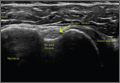
SAN DIEGO – Assessment of the trachea and pleura via point-of-care ultrasound is superior to auscultation in determining the exact location of the endotracheal tube, a randomized, single-center study found.
“It’s been reported that about 20% of the time the endotracheal tube is malpositioned,” study author Dr. Davinder S. Ramsingh said in an interview at the annual meeting of the American Society of Anesthesiologists. “Most of the time (the tube) is too deep, which can lead to severe complications.”

In a double-blinded, randomized study, Dr. Ramsingh and his associates assessed the accuracy of auscultation vs. point-of-care ultrasound in verifying the correct position of the endotracheal tube (ETT). They enrolled 42 adults who required general anesthesia with ETT and randomized them to right main bronchus, left main bronchus, or tracheal intubation, followed by fiber optically–guided visualization to place the ETT. Next, an anesthesiologist blinded to the ETT exact location used auscultation to assess the location of the ETT, while another anesthesiologist blinded to the ETT exact location used point-of-care ultrasound to assess the location of the ETT. The ultrasound exam consisted of assessing tracheal dilation via standard cuff inflation with air and evaluation of pleural lung sliding, explained Dr. Ramsingh of the department of anesthesiology and perioperative care at the University of California, Irvine.
Dr. Ramsingh reported that in differentiating tracheal versus bronchial intubations, auscultation demonstrated a sensitivity of 66% and a specificity of 59%, while ultrasound demonstrated a sensitivity of 93% and a specificity of 96%. Chi-square comparison showed a statistically significant improvement with ultrasound (P = .0005), while inter-observer agreement of the ultrasound findings was 100%.
Limitations of the study, he said, include the fact that “we don’t know the incidence of malpositioned endotracheal tubes in the operating room and that this study was evaluating patients undergoing elective surgical procedures.”
The researchers reported having no financial disclosures.
SAN DIEGO – Assessment of the trachea and pleura via point-of-care ultrasound is superior to auscultation in determining the exact location of the endotracheal tube, a randomized, single-center study found.
“It’s been reported that about 20% of the time the endotracheal tube is malpositioned,” study author Dr. Davinder S. Ramsingh said in an interview at the annual meeting of the American Society of Anesthesiologists. “Most of the time (the tube) is too deep, which can lead to severe complications.”
In a double-blinded, randomized study, Dr. Ramsingh and his associates assessed the accuracy of auscultation vs. point-of-care ultrasound in verifying the correct position of the endotracheal tube (ETT). They enrolled 42 adults who required general anesthesia with ETT and randomized them to right main bronchus, left main bronchus, or tracheal intubation, followed by fiber optically–guided visualization to place the ETT. Next, an anesthesiologist blinded to the ETT exact location used auscultation to assess the location of the ETT, while another anesthesiologist blinded to the ETT exact location used point-of-care ultrasound to assess the location of the ETT. The ultrasound exam consisted of assessing tracheal dilation via standard cuff inflation with air and evaluation of pleural lung sliding, explained Dr. Ramsingh of the department of anesthesiology and perioperative care at the University of California, Irvine.
Dr. Ramsingh reported that in differentiating tracheal versus bronchial intubations, auscultation demonstrated a sensitivity of 66% and a specificity of 59%, while ultrasound demonstrated a sensitivity of 93% and a specificity of 96%. Chi-square comparison showed a statistically significant improvement with ultrasound (P = .0005), while inter-observer agreement of the ultrasound findings was 100%.
Limitations of the study, he said, include the fact that “we don’t know the incidence of malpositioned endotracheal tubes in the operating room and that this study was evaluating patients undergoing elective surgical procedures.”
The researchers reported having no financial disclosures.
AT THE ASA ANNUAL MEETING
Key clinical point: Using point-of-care ultrasound was superior to auscultation in determining the exact location of the endotracheal tube.
Major finding: In differentiating tracheal versus bronchial intubations, auscultation demonstrated a sensitivity of 66% and a specificity of 59%, while ultrasound demonstrated a sensitivity of 93% and a specificity of 96%.
Data source: An randomized study of 42 adults who required general anesthesia with ETT.
Disclosures: The researchers reported having no financial disclosures.
Optical coherence tomography for PCI gets boost in OPINION trial
PARIS – The first-ever head-to-head randomized trial comparing clinical outcomes of optical coherence tomography and intravascular ultrasound (IVUS) for guidance of percutaneous coronary intervention with a second-generation drug-eluting stent has ended in a draw.
“The clinical outcomes in both OCT-guided PCI and IVUS-guided PCI were excellent in the OPINION study,” Dr. Takashi Kubo reported at the annual congress of the European Association of Percutaneous Cardiovascular Interventions.
The form of OCT used in this randomized trial is called optimal frequency domain imaging (OFDI). On the strength of the OPINION results, OFDI deserves to get an upgrade in the PCI treatment guidelines, said Dr. Kubo of Wakayama (Japan) University.
He noted that the 2014 European Society of Cardiology guidelines give IVUS a Class IIa recommendation in selected patients to optimize stent implantation, with a Level of Evidence of B (Eur Heart J. 2014 Oct 1;35:2541-619). The guidelines give OCT (optimal coherence tomography), the more recent and less-studied technology, a Class IIb, Level of Evidence C.
“Our results might influence the next ESC guidelines,” according to Dr. Kubo. “OCT use during PCI should have a Class IIa recommendation.”
The OPINION trial was a prospective, 42-site Japanese study in which 800 patients scheduled for PCI with the Terumo Nobori biolimus-eluting resorbable polymer stent were randomized to an OFDI- or IVUS-guided procedure. All participants underwent follow-up coronary angiography at 8 months and clinical assessment at 12 months.
The primary study endpoint was target vessel failure at 12 months post-PCI, a composite comprising cardiac death, target vessel–related MI, or clinically driven target vessel revascularization. The rate was 5.2% in the OFDI group and statistically similar at 4.9% in the IVUS arm. No cases of contrast-induced nephropathy occurred in either study arm, and stroke rates in both groups were similarly low.
Also noteworthy was the finding that the two intracoronary imaging technologies resulted in similar rates of procedural change: 38% of patients in the OFDI group had a procedural change as result of the imaging findings, as did 36% of the IVUS group. Examples of these procedural changes included upsizing the pre- or postdilatation balloon size or pressure, addition of an another stent, or the use of a distal protection device.
In Japan, where both OCT and IVUS during PCI are routinely reimbursed, roughly 80% of PCI patients undergo one of the two intracoronary imaging procedures. In the United States and Europe, the situation is reversed, Dr. Kubo observed.
Discussant Dr. Ron Waksman agreed with Dr. Kubo that the OPINION results warrant reconsideration of OCT’s Class IIb recommendation in the ESC PCI guidelines. But he thinks the study has a major limitation.
“In my view, this was a missed opportunity to include an angiographically guided PCI arm to establish the superiority of invasive imaging over angiographically guided PCI,” said Dr. Waksman of the MedStar Heart Institute in Washington. While he noted that a recent meta-analysis of 20 studies in more than 29,000 patients concluded that IVUS-guided implantation of drug-eluting stents was associated with a 38% reduction in the risk of mortality, a 23% decrease in major adverse cardiovascular events, and a 41% reduction in stent thrombosis, compared with angiographically guided PCI (BMC Cardiovasc Disord. 2015 Nov 17;15:153), given the inherent limitations of meta-analyses he’s not convinced that cardiologists really need imaging guidance.
“ILUMIEN III, to my view, is the right study design because it randomizes patients to OCT guidance, IVUS guidance, or angiographic guidance to see if there are important differences. We will have to wait for the ILUMIEN III study results to prove the superiority of invasive imaging over angiographically guided PCI,” according to Dr. Waksman.
It’s anticipated that the ILUMIEN III trial will be ready for presentation at EuroPCR 2017.
The OPINION trial was sponsored by Terumo. Dr. Kubo is a consultant to and recipient of an institutional research grant from the company.
AT EUROPCR 2016
Key clinical point: A large, randomized trial shows PCI clinical outcomes are equivalent with optical coherence tomography and intravascular ultrasound guidance.
Major finding: The composite rate of cardiac death, target vessel–related MI, or clinically driven target vessel revascularization within 12 months of PCI was 5.2% in the group whose procedure was guided by optical coherence tomography and statistically similar at 4.9% in patients whose PCI was guided by intravascular ultrasound.
Data source: This was a randomized, prospective, multicenter, 12-month follow-up trial of 800 Japanese patients scheduled for PCI under intracoronary imaging guidance provided by either IVUS or OCT.
Disclosures: The OPINION trial was sponsored by Terumo. The study presenter is a consultant to and recipient of an institutional research grant from the company.

Linea Aspera as Rotational Landmark for Tumor Endoprostheses: A Computed Tomography Study
The distal or proximal femur with tumor endoprosthesis is commonly replaced after segmental resections for bone tumors, complex trauma, or revision arthroplasty. In conventional joint replacements, correct rotational alignment of the component is referenced off anatomical landmarks in the proximal or distal femur. After tumor resection, however, these landmarks are often not available for rotational orientation. There are no reports of studies validating a particular method of establishing rotation in these cases.
To establish a guide for rotational alignment of tumor endoprostheses, we set out to define the natural location of the linea aspera (LA) based on axial computed tomography (CT) scans. The LA is often the most outstanding visible bony landmark on a cross-section of the femur during surgery, and it would be helpful to know its normal orientation in relation to the true anteroposterior (AP) axis of the femur and to the femoral version. We wanted to answer these 5 questions:
1. Is the prominence of the LA easily identifiable on cross-section at different levels of the femoral shaft?
2. Does an axis passing through the LA correspond to the AP axis of the femur?
3. If not, is this axis offset internally or externally and by how much?
4. Is this offset constant at all levels of the femoral shaft?
5. How does the LA axis relate to the femoral neck axis at these levels?
The answers determine if the LA can be reliably used for rotational alignment of tumor endoprostheses.
Materials and Methods
After this study received Institutional Review Board approval, we retrospectively reviewed whole-body fluorine-18-deoxyglucose (FDG) positron emission tomography–computed tomography (PET-CT) studies performed in our hospital between 2003 and 2006 to identify those with full-length bilateral femur CT scans. These scans were available on the hospital’s computerized picture archiving system (General Electric). Patients could be included in the study as long as they were at least 18 years old at time of scan and did not have any pathology that deformed the femur, broke a cortex, or otherwise caused any gross asymmetry of the femur. Of the 72 patients with full-length femur CT scans, 3 were excluded: 1 with a congenital hip dysplasia, 1 with an old, malunited femoral fracture, and 1 who was 15 years old at time of scan.
Axial Slice Selection
For each patient, scout AP films were used to measure femoral shaft length from the top of the greater trochanter to the end of the lateral femoral condyle. The levels of the proximal third, midshaft, and distal third were then calculated based on this length. The LA was studied on the axial slices nearest these levels. Next, we scrolled through the scans to identify an axial slice that best showed the femoral neck axis. The literature on CT measurement of femoral anteversion is varied. Some articles describe a technique that uses 2 superimposed axial slices, and others describe a single axial slice.1-3 We used 1 axial slice to draw the femoral neck axis because our computer software could not superimpose 2 images on 1 screen and because the CT scans were not made under specific protocols to measure anteversion but rather were part of a cancer staging work-up. Axial cuts were made at 5-mm intervals, and not all scans included a single slice capturing the head, neck, and greater trochanter. Therefore, we used a (previously described) method in which the femoral neck axis is drawn on a slice that most captured the femoral neck, usually toward its base.4 Last, in order to draw the posterior condyle (PC) axis, we selected an axial slice that showed the posterior-most aspects of the femoral condyles at the intercondylar notch.
Determining Anteroposterior and Posterior Condyle Axes of Femur
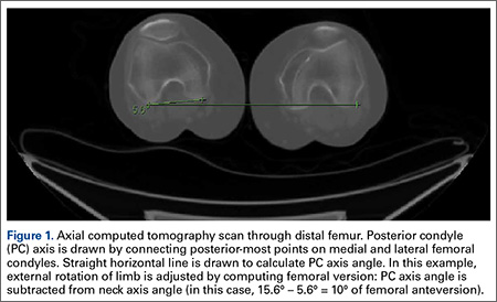
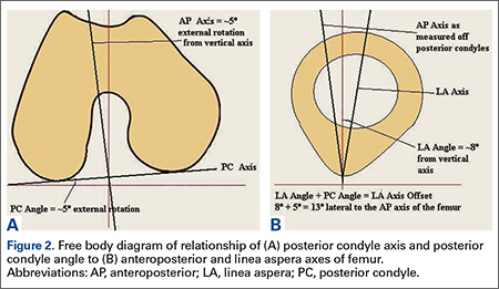
As we made all measurements for each femur off a single CT scan, we were able to use a straight horizontal line—drawn on-screen with a software tool—as a reference for measuring rotation. On a distal femur cut, the PC axis is drawn by connecting the posterior-most points of both condyles. The software calculates the angle formed—the PC angle (Figure 1). This angle, the degree to which the PC axis deviates from a straight horizontal line on-screen, can be used to account for gross rotation of the limb on comparison of images. The AP axis of the femur is the axis perpendicular to the PC axis. As such, the PC angle can also be used to determine degree of deviation of the AP axis from a straight vertical line on-screen. The AP axis was used when calculating the LA axis at the various levels of the femur (Figure 2).
Femoral Version
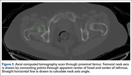
We used the software tool to draw the femoral neck axis. From the end of this line, a straight horizontal line is drawn on-screen (Figure 3). The software calculates the angle formed—the femoral neck axis angle. We assigned a positive value for a femoral head that pointed anteriorly on the image and a negative value for a head that pointed posteriorly. Adjusting for external rotation of the limb involved calculating the femoral version by subtracting the PC angle from the neck axis angle; adjusting for internal rotation involved adding these 2 angles.
Linea Aspera Morphology
After viewing the first 20 CT scans, we identified 3 types of LA morphology. Type I presents as a thickening on the posterior cortex with a sharp apex; type II presents as a flat-faced but distinct ridge of bone between the medial and lateral lips; and in type III there is no distinct cortical thickening with blunted medial and lateral lips; the latter is always more prominent.
Linea Aspera Axis Offset
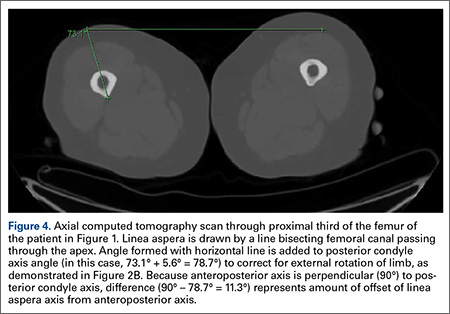
From the most posterior point of the LA, a line drawn forward bisecting the femoral canal defined the LA axis. In type I morphology, the posterior-most point was the apex; in type II, the middle of flat posterior surface was used as the starting point; in type III, the lateral lip was used, as it was sharper than the medial lip. This line is again referenced with a straight horizontal line across the image. The PC angle is then added to account for limb rotation, and the result is the LA angle. As the AP axis is perpendicular to the PC axis, the LA angle is subtracted from 90°; the difference represents the amount of offset of the LA axis from the AP axis. By convention, we assigned this a positive value for an LA lateral to the midpoint of the femur and a negative value for an LA medial to the midpoint (Figure 4).
Linea Aspera Axis and Femoral Neck Axis
The angle between the LA axis and the PC axis was measured. The femoral version angle was subtracted from that angle to obtain the arc between the LA axis and the femoral neck axis.
Statistical Analyses
All analyses were performed with SAS 9.1 (SAS Institute). All tests were 2-sided and conducted at the .05 significance level. No adjustments were made for multiple testing. Statistical analysis was performed with nonparametric tests and without making assumptions about the distribution of the study population. Univariate analyses were performed to test for significant side-to-side differences in femoral length, femoral version angle, and LA torsion angles at each level. A multivariate analysis was performed to test for interactions between sex, side, and level. In all analyses, P < .05 was used as the cutoff value for statistical significance.
Results
Femoral lengths varied by side and sex. The left side was longer than the right by a mean of 1.3 mm (P = .008). With multivariate analysis taking into account sex and age (cumulated per decade), there was still a significant effect of side on femoral length. Sex also had a significant effect on femoral length, with females’ femurs shorter by 21.7 mm (standard error, 5.0 mm). Mean (SD) anteversion of the femoral neck was 7.9° (12.7°) on the left and 13.3° (13.0°) on the right; the difference between sides was significant (P < .001). In a multivariate analysis performed to identify potential predictors of femoral version, side still had a significant (P < .001) independent effect; sex and age did not have an effect.
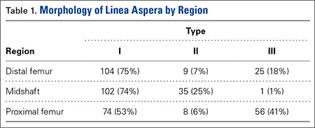
LA morphology varied according to femoral shaft level (Table 1). The morphology was type I in 75% of patients at the distal femur and 74% of patients at the midshaft femur, while only 53% of patients had a type I morphology at the proximal femur. The proportion of type III morphology was larger in the proximal femur (41%) than in the other locations.
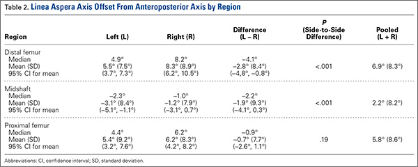
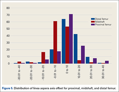
The LA axis of the femur did not correspond exactly to the AP axis at all femoral levels. At the distal femur, mean (SD) lateral offset of the LA axis was 5.5° (7.5°) on the left and 8.3° (8.9°) on the right. At the midshaft, mean (SD) medial offset of the LA axis was 3.1° (8.4°) on the left and 1.2° (7.9°) on the right. At the proximal femur, mean (SD) lateral offset of the LA axis was 5.4° (9.2°) on the left and 6.2° (8.3°) on the right. The side-to-side differences were statistically significant for the distal femur and midshaft but not the proximal femur. Table 2 lists the 95% confidence intervals for the mean values. As the range of differences was small (0.7°-2.8°), and the differences may not be clinically detected on gross inspection during surgery, we pooled both sides’ values to arrive at a single mean for each level. The LA axis was offset a mean (SD) of 6.9° (8.3°) laterally at the distal femur, 2.2° (8.2°) medially at the midshaft, and 5.8° (8.6°) laterally at the proximal femur. Figure 5 shows the frequency of distribution of LA axis offset.Offset of the LA axis from the AP axis of the femur was significantly (P < .001) different for each femoral level, even when a multivariate analysis was performed to determine the effect of sex, age, or side. Age and sex had no significant effect on mean offset of LA axis from AP axis.
We compared the mean arc between femoral neck axis and LA axis after referencing both off the PC axis. At the distal femur, mean (SD) arc between these 2 axes was 76.6° (13.1°) on the left and 68.3° (13.6°) on the right (mean difference, 8.3°); at the midshaft, mean (SD) arc was 85.2° (13.5°) on the left and 77.9° (13.1°) on the right (mean difference, 7.4°); at the proximal femur, mean (SD) arc was 76.7° (11.9°) on the left and 70.5° (12.8°) on the right (mean difference, 6.2°). The side-to-side differences were statistically significant (P < .001) for all locations.
In multivariate analysis, sex and age did not have an effect on mean arc between the 2 axes. Side and femoral level, however, had a significant effect (P < .001).
Discussion
In total hip arthroplasty, the goal is to restore femoral anteversion, usually referenced to the remaining femoral neck segment.3 In total knee arthroplasty (TKA), proper rotation preserves normal patellofemoral tracking.5 Various landmarks are used, such as the PCs or the epicondyles. After tumor resections, these landmarks are often lost.6 However, there are no reports of studies validating a particular method of achieving proper rotational orientation of tumor endoprostheses, though several methods are being used. One method involves inserting 2 drill bits before osteotomy—one proximal to the intended level of resection on the anterior femur, and the other on the anterior tibial shaft. The straight line formed can establish a plane of rotation (and length), which the surgeon must aim to restore when the components are placed. This method is useful for distal femur resections but not proximal femur resections. Another method, based on the LA’s anatomical position on the posterior aspect of the femur,4 uses the prominence of the LA to align the prosthesis. With this method, the LA is assumed to be directly posterior (6 o’clock) on the femur. However, this assumption has not been confirmed by any study. A third method, described by Heck and Carnesale,5 involves marking the anterior aspect of the femur after resection and aligning the components to it. The authors cautioned against using the LA as a landmark, saying that its course is highly variable.
The LA is a narrow, elevated length of bone, with medial and lateral lips, that serves as an attachment site for muscles in the posterior thigh. Proximally, the LA presents with lateral, medial, and intermediate lips. In the midshaft, it is often elevated by an underlying bony ridge or pilaster complex. Distally, it diverges into 2 ridges that form the triangular popliteal surface.1,7 For the LA to be a reliable landmark, first it must be clearly identifiable on viewing a femoral cross-section. The LA that presents with type I or II morphology is distinctly identifiable, and an axis from its apex and bisecting the canal can easily be constructed. In our study, the LA presented with type I or II morphology in 82% of distal femoral sections and 99% of midshaft femoral sections. Therefore, the LA is a conspicuous landmark at these levels. In the proximal femur, 59% had type I or II morphology. Type III morphology could be identified on cross-sections by the persisting prominence of the lateral lip. However, it may be difficult to appreciate the LA with this morphology at surgery.
Once the LA is identified, its normal cross-sectional position must be defined. One way to do this is to establish the relationship of its axis (LA axis) to the true AP axis. Based on mean values, the LA axis is laterally offset 7º at the distal third of the femur, medially offset 2º at the midshaft, and laterally offset 6º at the proximal third. Therefore, for ideal placement with the LA used for orientation, the component must be internally rotated 7º relative to the LA for femoral resection at the distal third, externally rotated 2º for resection at the midshaft, and internally rotated 6º for resection at the proximal third. Studies have demonstrated that joint contact forces and mechanical alignment of the lower limb can be altered with as little as 5º of femoral malrotation.8,9 Although such a small degree of malrotation is often asymptomatic, it can have long-term effects on soft-tissue tension and patellar tracking.10,11 Rotating-platform mobile-bearing TKA designs can compensate for femoral malrotation, but they may have little to no effect on patellar tracking.12 Therefore, we think aligning the components as near as possible to their natural orientation can prove beneficial in long-term patient management.
Another way of defining the normal cross-sectional position of the LA is to relate it to the femoral neck axis. We measured the difference between these 2 axes. Mean differences were 72º (distal femur), 81.5º (midshaft), and 73.5º (proximal third). Mean arc differences at all levels were larger on the left side—a reflection of the femoral neck being less anteverted on that side in our measurements. Standard deviations were smaller for measurements of LA axis offset from AP axis (range, 7.5°-9.2°) than for measurements of arc between LA axis and femoral neck axis (range, 11.9°-13.6°). This finding indicates there is less variation in the former method, making it preferable for defining the cross-sectional position of the LA.
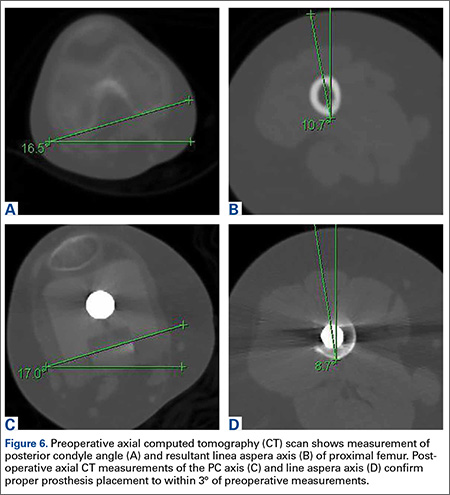
It has been said that the course of the LA is variable, and our data provide confirmation. The LA does not lie directly posterior (6 o’clock), and it does not trace a straight longitudinal course along the posterior femur, as demonstrated by the different LA axis offsets at 3 levels. However, we may still use it as a landmark if we remain aware how much the LA is offset from the AP axis at each femoral level. Figures 6A-6D, which show CT scans of a patient who underwent distal femoral resection and replacement with an endoprosthesis, illustrate how the LA axis was measured before surgery and how proper prosthesis placement was confirmed after surgery.
In hip arthroplasty, restoration of normal femoral version is the reference for endoprosthetic placement. The literature on “normal” femoral anteversion varies with the method used. In a review of studies on CT-measured adult femoral version, reported values ranged from 6.3° to 40°.2 Mean femoral version in our study ranged from 8° to 13°. Orthopedics textbooks generally put the value at 10° to 15º, and this seems to be the range that surgeons target.6 However, we found a statistically significant mean side-to-side difference of 5.4°. This finding is possibly explained by our large sample—it was larger than the samples used in other studies of CT-measured femoral version. Other studies have found mean side-to-side differences of up to 4.0º.5 Another explanation for our finding is that the studies may differ methodologically. The studies that established values for femoral anteversion were based on CT protocols—thinner slices (1-5 mm), use of foot holders to standardize limb rotation, use of 2 axial cuts in proximal femur to establish femoral neck axis2,13—designed specifically for this measurement. As the CT scans reviewed in our study are not designed for this purpose, errors in femoral version measurement may have been introduced, which may also explain why there is larger variation in measurements of the arc between the LA axis and the femoral neck axis.
Conclusion
The LA does not lie directly on the posterior surface of the femur. It deviates 6.9° laterally at the distal femur, 2.2° medially at the midshaft, and 6.9° laterally at the proximal third. As the LA is an easily identifiable structure on cross-sections of the femoral shaft at the midshaft and distal third of the femur, it may be useful as a rotational landmark for resections at these levels if these deviations are considered during tumor endoprosthetic replacements.
1. Desai SC, Willson S. Radiology of the linea aspera. Australas Radiol. 1985;29(3):273-274.
2. Kuo TY, Skedros JG, Bloebaum RD. Measurement of femoral anteversion by biplane radiography and computed tomography imaging: comparison with an anatomic reference. Invest Radiol. 2003;38(4):221-229.
3. Wines AP, McNicol D. Computed tomography measurement of the accuracy of component version in total hip arthroplasty. J Arthroplasty. 2006;21(5):696-701.
4. Gray H. Anatomy of the Human Body. Philadelphia, PA: Lea & Febiger; 1918.
5. Heck RK, Carnesale PG. General principles of tumors. In: Canale ST, ed. Campbell’s Operative Orthopaedics. Vol 1. 10th ed. St. Louis, MO: Mosby; 2003:733-791.
6. Katz, MA, Beck TD, Silber JS, Seldes RM, Lotke PA. Determining femoral rotational alignment in total knee arthroplasty: reliability of techniques. J Arthroplasty. 2001;16(3):301-305.
7. Pitt MJ. Radiology of the femoral linea aspera–pilaster complex: the track sign. Radiology. 1982;142(1):66.
8. Bretin P, O’Loughlin PF, Suero EM, et al. Influence of femoral malrotation on knee joint alignment and intra-articular contact pressures. Arch Orthop Trauma Surg. 2011;131(8):1115-1120.
9. Zihlmann MS, Stacoff A, Romero J, Quervain IK, Stüssi E. Biomechanical background and clinical observations of rotational malalignment in TKA: literature review and consequences. Clin Biomech. 2005;20(7):661-668.
10. Ghosh KM, Merican AM, Iranpour F, Deehan DJ, Amis AA. The effect of femoral component rotation on the extensor retinaculum of the knee. J Orthop Res. 2010;28(9):1136-1141.
11. Verlinden C, Uvin P, Labey L, Luyckx JP, Bellemans J, Vandenneucker H. The influence of malrotation of the femoral component in total knee replacement on the mechanics of patellofemoral contact during gait: an in vitro biomechanical study. J Bone Joint Surg Br. 2010;92(5):737-742.
12. Kessler O, Patil S, Colwell CW Jr, D’Lima DD. The effect of femoral component malrotation on patellar biomechanics. J Biomech. 2008;41(16):3332-3339.
13. Strecker W, Keppler P, Gebhard F, Kinzl L. Length and torsion of the lower limb. J Bone Joint Surg Br. 1997;79(6):1019-1023.
The distal or proximal femur with tumor endoprosthesis is commonly replaced after segmental resections for bone tumors, complex trauma, or revision arthroplasty. In conventional joint replacements, correct rotational alignment of the component is referenced off anatomical landmarks in the proximal or distal femur. After tumor resection, however, these landmarks are often not available for rotational orientation. There are no reports of studies validating a particular method of establishing rotation in these cases.
To establish a guide for rotational alignment of tumor endoprostheses, we set out to define the natural location of the linea aspera (LA) based on axial computed tomography (CT) scans. The LA is often the most outstanding visible bony landmark on a cross-section of the femur during surgery, and it would be helpful to know its normal orientation in relation to the true anteroposterior (AP) axis of the femur and to the femoral version. We wanted to answer these 5 questions:
1. Is the prominence of the LA easily identifiable on cross-section at different levels of the femoral shaft?
2. Does an axis passing through the LA correspond to the AP axis of the femur?
3. If not, is this axis offset internally or externally and by how much?
4. Is this offset constant at all levels of the femoral shaft?
5. How does the LA axis relate to the femoral neck axis at these levels?
The answers determine if the LA can be reliably used for rotational alignment of tumor endoprostheses.
Materials and Methods
After this study received Institutional Review Board approval, we retrospectively reviewed whole-body fluorine-18-deoxyglucose (FDG) positron emission tomography–computed tomography (PET-CT) studies performed in our hospital between 2003 and 2006 to identify those with full-length bilateral femur CT scans. These scans were available on the hospital’s computerized picture archiving system (General Electric). Patients could be included in the study as long as they were at least 18 years old at time of scan and did not have any pathology that deformed the femur, broke a cortex, or otherwise caused any gross asymmetry of the femur. Of the 72 patients with full-length femur CT scans, 3 were excluded: 1 with a congenital hip dysplasia, 1 with an old, malunited femoral fracture, and 1 who was 15 years old at time of scan.
Axial Slice Selection
For each patient, scout AP films were used to measure femoral shaft length from the top of the greater trochanter to the end of the lateral femoral condyle. The levels of the proximal third, midshaft, and distal third were then calculated based on this length. The LA was studied on the axial slices nearest these levels. Next, we scrolled through the scans to identify an axial slice that best showed the femoral neck axis. The literature on CT measurement of femoral anteversion is varied. Some articles describe a technique that uses 2 superimposed axial slices, and others describe a single axial slice.1-3 We used 1 axial slice to draw the femoral neck axis because our computer software could not superimpose 2 images on 1 screen and because the CT scans were not made under specific protocols to measure anteversion but rather were part of a cancer staging work-up. Axial cuts were made at 5-mm intervals, and not all scans included a single slice capturing the head, neck, and greater trochanter. Therefore, we used a (previously described) method in which the femoral neck axis is drawn on a slice that most captured the femoral neck, usually toward its base.4 Last, in order to draw the posterior condyle (PC) axis, we selected an axial slice that showed the posterior-most aspects of the femoral condyles at the intercondylar notch.
Determining Anteroposterior and Posterior Condyle Axes of Femur
As we made all measurements for each femur off a single CT scan, we were able to use a straight horizontal line—drawn on-screen with a software tool—as a reference for measuring rotation. On a distal femur cut, the PC axis is drawn by connecting the posterior-most points of both condyles. The software calculates the angle formed—the PC angle (Figure 1). This angle, the degree to which the PC axis deviates from a straight horizontal line on-screen, can be used to account for gross rotation of the limb on comparison of images. The AP axis of the femur is the axis perpendicular to the PC axis. As such, the PC angle can also be used to determine degree of deviation of the AP axis from a straight vertical line on-screen. The AP axis was used when calculating the LA axis at the various levels of the femur (Figure 2).
Femoral Version
We used the software tool to draw the femoral neck axis. From the end of this line, a straight horizontal line is drawn on-screen (Figure 3). The software calculates the angle formed—the femoral neck axis angle. We assigned a positive value for a femoral head that pointed anteriorly on the image and a negative value for a head that pointed posteriorly. Adjusting for external rotation of the limb involved calculating the femoral version by subtracting the PC angle from the neck axis angle; adjusting for internal rotation involved adding these 2 angles.
Linea Aspera Morphology
After viewing the first 20 CT scans, we identified 3 types of LA morphology. Type I presents as a thickening on the posterior cortex with a sharp apex; type II presents as a flat-faced but distinct ridge of bone between the medial and lateral lips; and in type III there is no distinct cortical thickening with blunted medial and lateral lips; the latter is always more prominent.
Linea Aspera Axis Offset
From the most posterior point of the LA, a line drawn forward bisecting the femoral canal defined the LA axis. In type I morphology, the posterior-most point was the apex; in type II, the middle of flat posterior surface was used as the starting point; in type III, the lateral lip was used, as it was sharper than the medial lip. This line is again referenced with a straight horizontal line across the image. The PC angle is then added to account for limb rotation, and the result is the LA angle. As the AP axis is perpendicular to the PC axis, the LA angle is subtracted from 90°; the difference represents the amount of offset of the LA axis from the AP axis. By convention, we assigned this a positive value for an LA lateral to the midpoint of the femur and a negative value for an LA medial to the midpoint (Figure 4).
Linea Aspera Axis and Femoral Neck Axis
The angle between the LA axis and the PC axis was measured. The femoral version angle was subtracted from that angle to obtain the arc between the LA axis and the femoral neck axis.
Statistical Analyses
All analyses were performed with SAS 9.1 (SAS Institute). All tests were 2-sided and conducted at the .05 significance level. No adjustments were made for multiple testing. Statistical analysis was performed with nonparametric tests and without making assumptions about the distribution of the study population. Univariate analyses were performed to test for significant side-to-side differences in femoral length, femoral version angle, and LA torsion angles at each level. A multivariate analysis was performed to test for interactions between sex, side, and level. In all analyses, P < .05 was used as the cutoff value for statistical significance.
Results
Femoral lengths varied by side and sex. The left side was longer than the right by a mean of 1.3 mm (P = .008). With multivariate analysis taking into account sex and age (cumulated per decade), there was still a significant effect of side on femoral length. Sex also had a significant effect on femoral length, with females’ femurs shorter by 21.7 mm (standard error, 5.0 mm). Mean (SD) anteversion of the femoral neck was 7.9° (12.7°) on the left and 13.3° (13.0°) on the right; the difference between sides was significant (P < .001). In a multivariate analysis performed to identify potential predictors of femoral version, side still had a significant (P < .001) independent effect; sex and age did not have an effect.
LA morphology varied according to femoral shaft level (Table 1). The morphology was type I in 75% of patients at the distal femur and 74% of patients at the midshaft femur, while only 53% of patients had a type I morphology at the proximal femur. The proportion of type III morphology was larger in the proximal femur (41%) than in the other locations.
The LA axis of the femur did not correspond exactly to the AP axis at all femoral levels. At the distal femur, mean (SD) lateral offset of the LA axis was 5.5° (7.5°) on the left and 8.3° (8.9°) on the right. At the midshaft, mean (SD) medial offset of the LA axis was 3.1° (8.4°) on the left and 1.2° (7.9°) on the right. At the proximal femur, mean (SD) lateral offset of the LA axis was 5.4° (9.2°) on the left and 6.2° (8.3°) on the right. The side-to-side differences were statistically significant for the distal femur and midshaft but not the proximal femur. Table 2 lists the 95% confidence intervals for the mean values. As the range of differences was small (0.7°-2.8°), and the differences may not be clinically detected on gross inspection during surgery, we pooled both sides’ values to arrive at a single mean for each level. The LA axis was offset a mean (SD) of 6.9° (8.3°) laterally at the distal femur, 2.2° (8.2°) medially at the midshaft, and 5.8° (8.6°) laterally at the proximal femur. Figure 5 shows the frequency of distribution of LA axis offset.Offset of the LA axis from the AP axis of the femur was significantly (P < .001) different for each femoral level, even when a multivariate analysis was performed to determine the effect of sex, age, or side. Age and sex had no significant effect on mean offset of LA axis from AP axis.
We compared the mean arc between femoral neck axis and LA axis after referencing both off the PC axis. At the distal femur, mean (SD) arc between these 2 axes was 76.6° (13.1°) on the left and 68.3° (13.6°) on the right (mean difference, 8.3°); at the midshaft, mean (SD) arc was 85.2° (13.5°) on the left and 77.9° (13.1°) on the right (mean difference, 7.4°); at the proximal femur, mean (SD) arc was 76.7° (11.9°) on the left and 70.5° (12.8°) on the right (mean difference, 6.2°). The side-to-side differences were statistically significant (P < .001) for all locations.
In multivariate analysis, sex and age did not have an effect on mean arc between the 2 axes. Side and femoral level, however, had a significant effect (P < .001).
Discussion
In total hip arthroplasty, the goal is to restore femoral anteversion, usually referenced to the remaining femoral neck segment.3 In total knee arthroplasty (TKA), proper rotation preserves normal patellofemoral tracking.5 Various landmarks are used, such as the PCs or the epicondyles. After tumor resections, these landmarks are often lost.6 However, there are no reports of studies validating a particular method of achieving proper rotational orientation of tumor endoprostheses, though several methods are being used. One method involves inserting 2 drill bits before osteotomy—one proximal to the intended level of resection on the anterior femur, and the other on the anterior tibial shaft. The straight line formed can establish a plane of rotation (and length), which the surgeon must aim to restore when the components are placed. This method is useful for distal femur resections but not proximal femur resections. Another method, based on the LA’s anatomical position on the posterior aspect of the femur,4 uses the prominence of the LA to align the prosthesis. With this method, the LA is assumed to be directly posterior (6 o’clock) on the femur. However, this assumption has not been confirmed by any study. A third method, described by Heck and Carnesale,5 involves marking the anterior aspect of the femur after resection and aligning the components to it. The authors cautioned against using the LA as a landmark, saying that its course is highly variable.
The LA is a narrow, elevated length of bone, with medial and lateral lips, that serves as an attachment site for muscles in the posterior thigh. Proximally, the LA presents with lateral, medial, and intermediate lips. In the midshaft, it is often elevated by an underlying bony ridge or pilaster complex. Distally, it diverges into 2 ridges that form the triangular popliteal surface.1,7 For the LA to be a reliable landmark, first it must be clearly identifiable on viewing a femoral cross-section. The LA that presents with type I or II morphology is distinctly identifiable, and an axis from its apex and bisecting the canal can easily be constructed. In our study, the LA presented with type I or II morphology in 82% of distal femoral sections and 99% of midshaft femoral sections. Therefore, the LA is a conspicuous landmark at these levels. In the proximal femur, 59% had type I or II morphology. Type III morphology could be identified on cross-sections by the persisting prominence of the lateral lip. However, it may be difficult to appreciate the LA with this morphology at surgery.
Once the LA is identified, its normal cross-sectional position must be defined. One way to do this is to establish the relationship of its axis (LA axis) to the true AP axis. Based on mean values, the LA axis is laterally offset 7º at the distal third of the femur, medially offset 2º at the midshaft, and laterally offset 6º at the proximal third. Therefore, for ideal placement with the LA used for orientation, the component must be internally rotated 7º relative to the LA for femoral resection at the distal third, externally rotated 2º for resection at the midshaft, and internally rotated 6º for resection at the proximal third. Studies have demonstrated that joint contact forces and mechanical alignment of the lower limb can be altered with as little as 5º of femoral malrotation.8,9 Although such a small degree of malrotation is often asymptomatic, it can have long-term effects on soft-tissue tension and patellar tracking.10,11 Rotating-platform mobile-bearing TKA designs can compensate for femoral malrotation, but they may have little to no effect on patellar tracking.12 Therefore, we think aligning the components as near as possible to their natural orientation can prove beneficial in long-term patient management.
Another way of defining the normal cross-sectional position of the LA is to relate it to the femoral neck axis. We measured the difference between these 2 axes. Mean differences were 72º (distal femur), 81.5º (midshaft), and 73.5º (proximal third). Mean arc differences at all levels were larger on the left side—a reflection of the femoral neck being less anteverted on that side in our measurements. Standard deviations were smaller for measurements of LA axis offset from AP axis (range, 7.5°-9.2°) than for measurements of arc between LA axis and femoral neck axis (range, 11.9°-13.6°). This finding indicates there is less variation in the former method, making it preferable for defining the cross-sectional position of the LA.
It has been said that the course of the LA is variable, and our data provide confirmation. The LA does not lie directly posterior (6 o’clock), and it does not trace a straight longitudinal course along the posterior femur, as demonstrated by the different LA axis offsets at 3 levels. However, we may still use it as a landmark if we remain aware how much the LA is offset from the AP axis at each femoral level. Figures 6A-6D, which show CT scans of a patient who underwent distal femoral resection and replacement with an endoprosthesis, illustrate how the LA axis was measured before surgery and how proper prosthesis placement was confirmed after surgery.
In hip arthroplasty, restoration of normal femoral version is the reference for endoprosthetic placement. The literature on “normal” femoral anteversion varies with the method used. In a review of studies on CT-measured adult femoral version, reported values ranged from 6.3° to 40°.2 Mean femoral version in our study ranged from 8° to 13°. Orthopedics textbooks generally put the value at 10° to 15º, and this seems to be the range that surgeons target.6 However, we found a statistically significant mean side-to-side difference of 5.4°. This finding is possibly explained by our large sample—it was larger than the samples used in other studies of CT-measured femoral version. Other studies have found mean side-to-side differences of up to 4.0º.5 Another explanation for our finding is that the studies may differ methodologically. The studies that established values for femoral anteversion were based on CT protocols—thinner slices (1-5 mm), use of foot holders to standardize limb rotation, use of 2 axial cuts in proximal femur to establish femoral neck axis2,13—designed specifically for this measurement. As the CT scans reviewed in our study are not designed for this purpose, errors in femoral version measurement may have been introduced, which may also explain why there is larger variation in measurements of the arc between the LA axis and the femoral neck axis.
Conclusion
The LA does not lie directly on the posterior surface of the femur. It deviates 6.9° laterally at the distal femur, 2.2° medially at the midshaft, and 6.9° laterally at the proximal third. As the LA is an easily identifiable structure on cross-sections of the femoral shaft at the midshaft and distal third of the femur, it may be useful as a rotational landmark for resections at these levels if these deviations are considered during tumor endoprosthetic replacements.
1. Desai SC, Willson S. Radiology of the linea aspera. Australas Radiol. 1985;29(3):273-274.
2. Kuo TY, Skedros JG, Bloebaum RD. Measurement of femoral anteversion by biplane radiography and computed tomography imaging: comparison with an anatomic reference. Invest Radiol. 2003;38(4):221-229.
3. Wines AP, McNicol D. Computed tomography measurement of the accuracy of component version in total hip arthroplasty. J Arthroplasty. 2006;21(5):696-701.
4. Gray H. Anatomy of the Human Body. Philadelphia, PA: Lea & Febiger; 1918.
5. Heck RK, Carnesale PG. General principles of tumors. In: Canale ST, ed. Campbell’s Operative Orthopaedics. Vol 1. 10th ed. St. Louis, MO: Mosby; 2003:733-791.
6. Katz, MA, Beck TD, Silber JS, Seldes RM, Lotke PA. Determining femoral rotational alignment in total knee arthroplasty: reliability of techniques. J Arthroplasty. 2001;16(3):301-305.
7. Pitt MJ. Radiology of the femoral linea aspera–pilaster complex: the track sign. Radiology. 1982;142(1):66.
8. Bretin P, O’Loughlin PF, Suero EM, et al. Influence of femoral malrotation on knee joint alignment and intra-articular contact pressures. Arch Orthop Trauma Surg. 2011;131(8):1115-1120.
9. Zihlmann MS, Stacoff A, Romero J, Quervain IK, Stüssi E. Biomechanical background and clinical observations of rotational malalignment in TKA: literature review and consequences. Clin Biomech. 2005;20(7):661-668.
10. Ghosh KM, Merican AM, Iranpour F, Deehan DJ, Amis AA. The effect of femoral component rotation on the extensor retinaculum of the knee. J Orthop Res. 2010;28(9):1136-1141.
11. Verlinden C, Uvin P, Labey L, Luyckx JP, Bellemans J, Vandenneucker H. The influence of malrotation of the femoral component in total knee replacement on the mechanics of patellofemoral contact during gait: an in vitro biomechanical study. J Bone Joint Surg Br. 2010;92(5):737-742.
12. Kessler O, Patil S, Colwell CW Jr, D’Lima DD. The effect of femoral component malrotation on patellar biomechanics. J Biomech. 2008;41(16):3332-3339.
13. Strecker W, Keppler P, Gebhard F, Kinzl L. Length and torsion of the lower limb. J Bone Joint Surg Br. 1997;79(6):1019-1023.
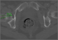
Emergency Imaging: Right hallux pain
A 55-year-old man presented with a 2-day history of acute first toe pain in his right foot after banging the affected toe on a door. Physical examination demonstrated a swollen first toe with marked tenderness to palpation. Radiographs were obtained (Figures 1a and 1b).
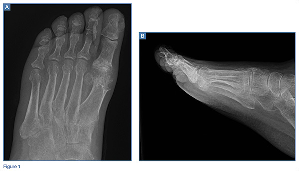
What is the diagnosis? What additional imaging tests may be useful to confirm the diagnosis?
Answer
The radiographs of the right foot excluded fracture as the underlying etiology of the patient’s pain. The findings included soft tissue swelling and periarticular (ie, near but not involving the joint) erosions involving the first metatarsal head (white asterisks, Figure 1c). The erosion on the medial aspect of the metatarsal head had remodeling of bone at the periphery of the erosion, which created the appearance of “overhanging edges” (white arrows, Figure 1c). The radiographic appearance suggests the diagnosis of gouty arthritis.
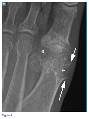
Gouty arthritis, which is caused by the deposition of monosodium urate crystals in the soft tissues surrounding joints, continues to increase in prevalence—likely due to the growing aging population and risk factors such as obesity and diabetes. Gouty arthritis typically presents as painful episodes of arthritis affecting a single joint that can be extremely tender to touch. Acute attacks typically subside within 5 to 7 days. Acute gout may result in fever and elevated white blood cell counts, making it difficult to distinguish from septic arthritis.1 While more common in males in the younger population, gout affects men and women equally in patients older than age 60 years.2
While patients with gouty arthritis have hyperuricemia, only approximately 10% develop gout. The American College of Rheumatology’s preliminary criteria2 for the diagnosis of gout include the presence of characteristic urate crystals in the joint fluid of the affected joint during the attack, the presence of a tophus (soft tissue mass containing urate crystals), or at least six of the following:
- More than one attack of acute arthritis
- Maximum joint inflammation developed within 1 day
- Monoarticular arthritis
- Redness of the joint
- First metatarsophalangeal (MTP) joint pain/swelling
- Unilateral first MTP joint attack
- Unilateral tarsal joint attack
- Suspected tophus
- Hyperuricemia
- Asymmetrical swelling of the joint on radiography
- Subcortical cysts without erosions on radiography
- Joint fluid culture negative during an attack.
As highlighted by the criteria, the first MTP joint is a common location for gouty arthritis, and is referred to as podagra. A meta-analysis published in 2016 reports that an estimated 73% of patients with gout will have involvement of the first MTP.3
Regarding imaging studies, radiography is often the first imaging test performed to evaluate for gout, and can reveal characteristic findings such as periarticular erosions with sclerotic margins, overhanging edges of remodeling bone, and adjacent soft tissue tophi. These findings, however, occur late in the disease. Ultrasound may be useful for earlier diagnosis with the “double contour sign,” which is a specific finding representing the appearance of urate crystals deposited on the hyaline cartilage of the joint. Dual-energy computed tomography (CT) has been shown to not only demonstrate early erosions and soft tissue tophi, but also to characterize the crystals, making CT a highly sensitive and specific test for the detection of gouty arthritis.4
Treatment of acute episodes of gout includes nonsteroidal anti-inflammatory agents, colchicine, and corticosteroids. Early diagnosis and treatment can prevent progression to advanced arthritis and chronic impairment.
1. Eggebeen AT. Gout: an update. Am Fam Physician. 2007;76(6):801-808.
2. Wallace SL, Robinson H, Masi AT, Decker JL, McCarty DJ, Yü TF. Preliminary criteria for the classification of the acute arthritis of primary gout. Arthritis Rheum. 1977;20(3):895-900.
3. Stewart S, Dalbeth N, Vandal AC, Rome K. The first metatarsophalangeal joint in gout: a systematic review and meta-analyis. BMC Musculoskelet Disord. 2016;17(1):69.
4. Girish G, Glazebrook KN, Jacobson JA. Advanced imaging in gout. AJR Am J Roentgenol. 2013;201(3):515-525.
A 55-year-old man presented with a 2-day history of acute first toe pain in his right foot after banging the affected toe on a door. Physical examination demonstrated a swollen first toe with marked tenderness to palpation. Radiographs were obtained (Figures 1a and 1b).
What is the diagnosis? What additional imaging tests may be useful to confirm the diagnosis?
Answer
The radiographs of the right foot excluded fracture as the underlying etiology of the patient’s pain. The findings included soft tissue swelling and periarticular (ie, near but not involving the joint) erosions involving the first metatarsal head (white asterisks, Figure 1c). The erosion on the medial aspect of the metatarsal head had remodeling of bone at the periphery of the erosion, which created the appearance of “overhanging edges” (white arrows, Figure 1c). The radiographic appearance suggests the diagnosis of gouty arthritis.
Gouty arthritis, which is caused by the deposition of monosodium urate crystals in the soft tissues surrounding joints, continues to increase in prevalence—likely due to the growing aging population and risk factors such as obesity and diabetes. Gouty arthritis typically presents as painful episodes of arthritis affecting a single joint that can be extremely tender to touch. Acute attacks typically subside within 5 to 7 days. Acute gout may result in fever and elevated white blood cell counts, making it difficult to distinguish from septic arthritis.1 While more common in males in the younger population, gout affects men and women equally in patients older than age 60 years.2
While patients with gouty arthritis have hyperuricemia, only approximately 10% develop gout. The American College of Rheumatology’s preliminary criteria2 for the diagnosis of gout include the presence of characteristic urate crystals in the joint fluid of the affected joint during the attack, the presence of a tophus (soft tissue mass containing urate crystals), or at least six of the following:
- More than one attack of acute arthritis
- Maximum joint inflammation developed within 1 day
- Monoarticular arthritis
- Redness of the joint
- First metatarsophalangeal (MTP) joint pain/swelling
- Unilateral first MTP joint attack
- Unilateral tarsal joint attack
- Suspected tophus
- Hyperuricemia
- Asymmetrical swelling of the joint on radiography
- Subcortical cysts without erosions on radiography
- Joint fluid culture negative during an attack.
As highlighted by the criteria, the first MTP joint is a common location for gouty arthritis, and is referred to as podagra. A meta-analysis published in 2016 reports that an estimated 73% of patients with gout will have involvement of the first MTP.3
Regarding imaging studies, radiography is often the first imaging test performed to evaluate for gout, and can reveal characteristic findings such as periarticular erosions with sclerotic margins, overhanging edges of remodeling bone, and adjacent soft tissue tophi. These findings, however, occur late in the disease. Ultrasound may be useful for earlier diagnosis with the “double contour sign,” which is a specific finding representing the appearance of urate crystals deposited on the hyaline cartilage of the joint. Dual-energy computed tomography (CT) has been shown to not only demonstrate early erosions and soft tissue tophi, but also to characterize the crystals, making CT a highly sensitive and specific test for the detection of gouty arthritis.4
Treatment of acute episodes of gout includes nonsteroidal anti-inflammatory agents, colchicine, and corticosteroids. Early diagnosis and treatment can prevent progression to advanced arthritis and chronic impairment.
1. Eggebeen AT. Gout: an update. Am Fam Physician. 2007;76(6):801-808.
2. Wallace SL, Robinson H, Masi AT, Decker JL, McCarty DJ, Yü TF. Preliminary criteria for the classification of the acute arthritis of primary gout. Arthritis Rheum. 1977;20(3):895-900.
3. Stewart S, Dalbeth N, Vandal AC, Rome K. The first metatarsophalangeal joint in gout: a systematic review and meta-analyis. BMC Musculoskelet Disord. 2016;17(1):69.
4. Girish G, Glazebrook KN, Jacobson JA. Advanced imaging in gout. AJR Am J Roentgenol. 2013;201(3):515-525.
When does chest CT require contrast enhancement?
Computed tomography (CT) plays an important role in the diagnosis and treatment of many clinical conditions1 involving the chest wall, mediastinum, pleura, pulmonary arteries, and lung parenchyma. The need for enhancement with intravenous (IV) contrast depends on the specific clinical indication (Table 1).
EVALUATION OF SUSPECTED CANCER
CT is commonly used to diagnose, stage, and plan treatment for lung cancer, other primary neoplastic processes involving the chest, and metastatic disease.2 The need for contrast varies on a case-by-case basis, and the benefits of contrast should be weighed against the potential risks in each patient.
When the neoplasm has CT attenuation similar to that of adjacent structures (lymph nodes in the hilum, masses in the mediastinum or chest wall), IV contrast can improve identification of the lesion and delineation of its margins and the relationship with adjacent structures (eg, vascular structures) (Figure 1).
CT without contrast for screening
The diagnostic algorithm for lung cancer screening is evolving. The US Preventive Services Task Force currently recommends low-dose CT without contrast, along with appropriate patient counseling, for patients with a history of smoking and an age range as detailed in the Task Force statement.3
Follow-up of a solitary pulmonary nodule also typically does not require contrast enhancement, though some investigators have reported high sensitivity with dynamic contrast enhancement of pulmonary nodules.4 This represents a rare clinical application of chest CT with and without contrast.
EVALUATION OF THORACIC VASCULAR DISEASE
For the assessment of vascular disease, CT in most cases requires IV contrast to delineate the vessel lumen. Pulmonary embolic disease is the third most common cause of acute cardiovascular disease.5 CT pulmonary angiography is the most common way to assess for pulmonary embolic disease, as it is accurate, fast, and widely available, and can assess alternate pathologies in cases of undifferentiated chest pain. Contrast enhancement of the pulmonary arteries is key, as embolic disease is identified as abnormal filling defects within the pulmonary arteries (Figure 2).
Contrast enhancement is also used to evaluate superior vena cava syndrome. At our institution, the CT protocol includes concomitant injections in the upper-extremity veins, with imaging timed for venous phase enhancement (pulmonary venogram). In cases of suspected arteriovenous malformation, a protocol similar to that used for suspected pulmonary embolus is used (Figure 3), although in some instances, the imaging features of arteriovenous malformation may be detectable without IV contrast.
EVALUATION OF PULMONARY PARENCHYMAL DISEASE
Infection, inflammation, and edema of the lung parenchyma are usually well depicted on CT without contrast enhancement. However, contrast may be helpful if there are concerns about complications such as chest wall involvement, where contrast enhancement may help further delineate the extent of complications.
Assessment of interstitial lung disease does not require use of IV contrast; rather, a tailored protocol with thinner slices and noncontiguous expiratory images can be used to evaluate for air-trapping and dynamic airway compromise (Figure 4). Evaluation of chronic obstructive pulmonary disease also does not require IV contrast.
EVALUATION OF THE PLEURA
In pleural effusion, CT assessment for the presence, location, and extent of the effusion does not require contrast. However, contrast enhancement is used to evaluate suspected or known exudative effusions and empyema.6 It also aids the evaluation of metastatic or primary malignancy of the pleura, particularly in cases of occult disease, as enhancement and thickening of the pleura are of diagnostic interest.
EVALUATION OF AIRWAY DISEASE
Diseases of the large airway, such as stenosis and thickening, and diseases of the small airways, such as bronchiolitis, typically do not require contrast enhancement. At our institution, to assess dynamic airway narrowing, we use a dedicated airway protocol, including inspiratory and expiratory phases and multiplanar reformatted images.
EVALUATION OF STERNAL AND MEDIASTINAL INFECTIONS
Postoperative sternal wound infections are not uncommon and range from cellulitis to frank osteomyelitis. Mediastinitis may likewise be iatrogenic or may spread from the oropharynx. CT with contrast can help to depict infection of the chest wall or mediastinum and in some instances can also delineate the route of spread.7
TYPES OF IV CONTRAST MEDIA
Contrast media used in CT contain iodine, which causes increased absorption and scattering of radiation in body tissues and blood. Other contrast media, such as those used for magnetic resonance imaging or barium enemas, do not contain iodine. This absorption and scattering in turn results in higher CT attenuation values, or “enhancement” on CT images. The extent of enhancement depends on the amount and rate of contrast material administered, as well as on patient factors (eg, tissue vascularity, permeability, interstitial space) and the energy (tube voltage) of the incident x-rays.8
Adverse reactions
Contrast materials are generally safe; however, as with any pharmaceutical, there is the potential for adverse reactions. These reactions are relatively rare and are usually mild but occasionally can be severe.9 Anaphylactoid reactions have an unclear etiology but mimic allergic reactions, and they are more likely to occur in patients with a previous reaction to contrast and in patients with asthma or cardiovascular or renal disease.
Nonanaphylactoid reactions are dependent on contrast osmolality and on the volume and route of injection (unlike anaphylactoid reactions).10 Typical symptoms include warmth, metallic taste, and nausea or vomiting.
Contrast-related nephrotoxicity has been reported,11 although this has been challenged more recently.12 Suspected risk factors for this complication include advanced age, cardiovascular disease, treatment with chemotherapy, elevated serum creatinine level, dehydration, diabetes, use of nonsteroidal anti-inflammatory medications, myeloma,13 renal disease, and kidney transplant.
Detailed protocols for premedication and management of contrast adverse reactions are beyond the scope of this review and the reader is advised to refer to dedicated manuals.10
Acknowledgment: We are grateful for the editorial assistance of Megan M. Griffiths, scientific writer for the Imaging Institute, Cleveland Clinic.
- Rubin GD. Computed tomography: revolutionizing the practice of medicine for 40 years. Radiology 2014; 273(suppl 2):S45–S74.
- American College of Radiology. ACR-SCBT-MR-SPR practice parameter for the performance of thoracic computed tomography (CT). www.acr.org/~/media/ACR/Documents/PGTS/guidelines/CT_Thoracic.pdf. Accessed March 30, 2016.
- Moyer VA; US Preventive Services Task Force. Screening for lung cancer: US Preventive Services Task Force recommendation statement. Ann Intern Med 2014; 160:330–338.
- Yi CA, Lee KS, Kim EA, et al. Solitary pulmonary nodules: dynamic enhanced multi-detector row CT study and comparison with vascular endothelial growth factor and microvessel density. Radiology 2004; 233:191–199.
- Bolen MA, Renapurkar RD, Popovic ZB, et al. High-pitch ECG-synchronized pulmonary CT angiography versus standard CT pulmonary angiography: a prospective randomized study. AJR Am J Roentgenol 2013; 201:971–976.
- Kraus GJ. The split pleura sign. Radiology 2007; 243:297–298.
- Bae KT. Intravenous contrast medium administration and scan timing at CT: considerations and approaches. Radiology 2010; 256:32–61.
- Capps EF, Kinsella JJ, Gupta M, Bhatki AM, Opatowsky MJ. Emergency imaging assessment of acute, nontraumatic conditions of the head and neck. Radiographics 2010; 30:1335–1352.
- Singh J, Daftary A. Iodinated contrast media and their adverse reactions. J Nucl Med Technol 2008; 36:69–74.
- ACR Committee on Drugs and Contrast Media. ACR Manual on Contrast Media. Version 10.1. 2015. www.acr.org/~/media/37D84428BF1D4E1B9A3A2918DA9E27A3.pdf. Accessed March 29, 2016.
- Barrett BJ. Contrast nephrotoxicity. J Am Soc Nephrol 1994; 5:125–137.
- McDonald RJ, McDonald JS, Carter RE, et al. Intravenous contrast material exposure is not an independent risk factor for dialysis or mortality. Radiology 2014; 273:714–725.
- McCarthy CS, Becker JA. Multiple myeloma and contrast media. Radiology 1992; 183:519–521.
Computed tomography (CT) plays an important role in the diagnosis and treatment of many clinical conditions1 involving the chest wall, mediastinum, pleura, pulmonary arteries, and lung parenchyma. The need for enhancement with intravenous (IV) contrast depends on the specific clinical indication (Table 1).
EVALUATION OF SUSPECTED CANCER
CT is commonly used to diagnose, stage, and plan treatment for lung cancer, other primary neoplastic processes involving the chest, and metastatic disease.2 The need for contrast varies on a case-by-case basis, and the benefits of contrast should be weighed against the potential risks in each patient.
When the neoplasm has CT attenuation similar to that of adjacent structures (lymph nodes in the hilum, masses in the mediastinum or chest wall), IV contrast can improve identification of the lesion and delineation of its margins and the relationship with adjacent structures (eg, vascular structures) (Figure 1).
CT without contrast for screening
The diagnostic algorithm for lung cancer screening is evolving. The US Preventive Services Task Force currently recommends low-dose CT without contrast, along with appropriate patient counseling, for patients with a history of smoking and an age range as detailed in the Task Force statement.3
Follow-up of a solitary pulmonary nodule also typically does not require contrast enhancement, though some investigators have reported high sensitivity with dynamic contrast enhancement of pulmonary nodules.4 This represents a rare clinical application of chest CT with and without contrast.
EVALUATION OF THORACIC VASCULAR DISEASE
For the assessment of vascular disease, CT in most cases requires IV contrast to delineate the vessel lumen. Pulmonary embolic disease is the third most common cause of acute cardiovascular disease.5 CT pulmonary angiography is the most common way to assess for pulmonary embolic disease, as it is accurate, fast, and widely available, and can assess alternate pathologies in cases of undifferentiated chest pain. Contrast enhancement of the pulmonary arteries is key, as embolic disease is identified as abnormal filling defects within the pulmonary arteries (Figure 2).
Contrast enhancement is also used to evaluate superior vena cava syndrome. At our institution, the CT protocol includes concomitant injections in the upper-extremity veins, with imaging timed for venous phase enhancement (pulmonary venogram). In cases of suspected arteriovenous malformation, a protocol similar to that used for suspected pulmonary embolus is used (Figure 3), although in some instances, the imaging features of arteriovenous malformation may be detectable without IV contrast.
EVALUATION OF PULMONARY PARENCHYMAL DISEASE
Infection, inflammation, and edema of the lung parenchyma are usually well depicted on CT without contrast enhancement. However, contrast may be helpful if there are concerns about complications such as chest wall involvement, where contrast enhancement may help further delineate the extent of complications.
Assessment of interstitial lung disease does not require use of IV contrast; rather, a tailored protocol with thinner slices and noncontiguous expiratory images can be used to evaluate for air-trapping and dynamic airway compromise (Figure 4). Evaluation of chronic obstructive pulmonary disease also does not require IV contrast.
EVALUATION OF THE PLEURA
In pleural effusion, CT assessment for the presence, location, and extent of the effusion does not require contrast. However, contrast enhancement is used to evaluate suspected or known exudative effusions and empyema.6 It also aids the evaluation of metastatic or primary malignancy of the pleura, particularly in cases of occult disease, as enhancement and thickening of the pleura are of diagnostic interest.
EVALUATION OF AIRWAY DISEASE
Diseases of the large airway, such as stenosis and thickening, and diseases of the small airways, such as bronchiolitis, typically do not require contrast enhancement. At our institution, to assess dynamic airway narrowing, we use a dedicated airway protocol, including inspiratory and expiratory phases and multiplanar reformatted images.
EVALUATION OF STERNAL AND MEDIASTINAL INFECTIONS
Postoperative sternal wound infections are not uncommon and range from cellulitis to frank osteomyelitis. Mediastinitis may likewise be iatrogenic or may spread from the oropharynx. CT with contrast can help to depict infection of the chest wall or mediastinum and in some instances can also delineate the route of spread.7
TYPES OF IV CONTRAST MEDIA
Contrast media used in CT contain iodine, which causes increased absorption and scattering of radiation in body tissues and blood. Other contrast media, such as those used for magnetic resonance imaging or barium enemas, do not contain iodine. This absorption and scattering in turn results in higher CT attenuation values, or “enhancement” on CT images. The extent of enhancement depends on the amount and rate of contrast material administered, as well as on patient factors (eg, tissue vascularity, permeability, interstitial space) and the energy (tube voltage) of the incident x-rays.8
Adverse reactions
Contrast materials are generally safe; however, as with any pharmaceutical, there is the potential for adverse reactions. These reactions are relatively rare and are usually mild but occasionally can be severe.9 Anaphylactoid reactions have an unclear etiology but mimic allergic reactions, and they are more likely to occur in patients with a previous reaction to contrast and in patients with asthma or cardiovascular or renal disease.
Nonanaphylactoid reactions are dependent on contrast osmolality and on the volume and route of injection (unlike anaphylactoid reactions).10 Typical symptoms include warmth, metallic taste, and nausea or vomiting.
Contrast-related nephrotoxicity has been reported,11 although this has been challenged more recently.12 Suspected risk factors for this complication include advanced age, cardiovascular disease, treatment with chemotherapy, elevated serum creatinine level, dehydration, diabetes, use of nonsteroidal anti-inflammatory medications, myeloma,13 renal disease, and kidney transplant.
Detailed protocols for premedication and management of contrast adverse reactions are beyond the scope of this review and the reader is advised to refer to dedicated manuals.10
Acknowledgment: We are grateful for the editorial assistance of Megan M. Griffiths, scientific writer for the Imaging Institute, Cleveland Clinic.
- Rubin GD. Computed tomography: revolutionizing the practice of medicine for 40 years. Radiology 2014; 273(suppl 2):S45–S74.
- American College of Radiology. ACR-SCBT-MR-SPR practice parameter for the performance of thoracic computed tomography (CT). www.acr.org/~/media/ACR/Documents/PGTS/guidelines/CT_Thoracic.pdf. Accessed March 30, 2016.
- Moyer VA; US Preventive Services Task Force. Screening for lung cancer: US Preventive Services Task Force recommendation statement. Ann Intern Med 2014; 160:330–338.
- Yi CA, Lee KS, Kim EA, et al. Solitary pulmonary nodules: dynamic enhanced multi-detector row CT study and comparison with vascular endothelial growth factor and microvessel density. Radiology 2004; 233:191–199.
- Bolen MA, Renapurkar RD, Popovic ZB, et al. High-pitch ECG-synchronized pulmonary CT angiography versus standard CT pulmonary angiography: a prospective randomized study. AJR Am J Roentgenol 2013; 201:971–976.
- Kraus GJ. The split pleura sign. Radiology 2007; 243:297–298.
- Bae KT. Intravenous contrast medium administration and scan timing at CT: considerations and approaches. Radiology 2010; 256:32–61.
- Capps EF, Kinsella JJ, Gupta M, Bhatki AM, Opatowsky MJ. Emergency imaging assessment of acute, nontraumatic conditions of the head and neck. Radiographics 2010; 30:1335–1352.
- Singh J, Daftary A. Iodinated contrast media and their adverse reactions. J Nucl Med Technol 2008; 36:69–74.
- ACR Committee on Drugs and Contrast Media. ACR Manual on Contrast Media. Version 10.1. 2015. www.acr.org/~/media/37D84428BF1D4E1B9A3A2918DA9E27A3.pdf. Accessed March 29, 2016.
- Barrett BJ. Contrast nephrotoxicity. J Am Soc Nephrol 1994; 5:125–137.
- McDonald RJ, McDonald JS, Carter RE, et al. Intravenous contrast material exposure is not an independent risk factor for dialysis or mortality. Radiology 2014; 273:714–725.
- McCarthy CS, Becker JA. Multiple myeloma and contrast media. Radiology 1992; 183:519–521.
Multiple linear subcutaneous nodules
A 34-year-old woman sought consultation at our clinic for an asymptomatic swelling on her right foot that had been growing very slowly over the last 15 years. She said she had presented to other healthcare facilities, but no diagnosis had been made and no treatment had been offered.
Examination revealed a linear swelling extending from the lower third to the mid-dorsal surface of the right foot (Figure 1). Palpation revealed multiple, closely set nodules arranged in a linear fashion. This finding along with the history raised the suspicion of neurofibroma and other conditions in the differential diagnosis, eg, pure neuritic Hansen disease, phaeohyphomycosis, and palisaded neutrophilic granulomatous dermatitis. The rest of the mucocutaneous examination results were normal. No café-au-lait spots, axillary freckling, or other swelling suggestive of neurofibroma was seen. She had no family history of mucocutaneous disease or other systemic disorder.
Because of the suspicion of neurofibromatosis, slit-lamp examination of the eyes was done to rule out Lisch nodules, a common feature of neurofibromatosis; the results were normal. Plain radiography of the right foot showed only soft-tissue swelling. Magnetic resonance imaging with contrast, done to determine the extent of the lesions, revealed multiple dumbbell-shaped lesions with homogeneous enhancement (Figure 2). Histopathologic study of a biopsy specimen of the lesions showed tumor cells in the dermis. The cells were long, with elongated nuclei with pointed ends, arranged in long and short fascicles—an appearance characteristic of neurofibroma. Areas of hypocellularity and hypercellularity were seen, and on S100 protein immunostaining, the tumor cells showed strong nuclear and cytoplasmic positivity (Figure 3).
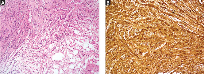
The histologic evaluation confirmed neurofibroma. The specific diagnosis of sporadic solitary neurofibroma was made based on the onset of the lesions, the number of lesions (one in this patient), and the absence of features suggestive of neurofibromatosis.
SPORADIC SOLITARY NEUROFIBROMA
Neurofibroma is a common tumor of the peripheral nerve sheath and, when present with features such as café-au-lait spots, axillary freckling, and characteristic bone changes, it is pathognomic of neurofibromatosis type 1.1 But solitary neurofibromas can occur sporadically in the absence of other features of neurofibromatosis.
Sporadic solitary neurofibroma arises from small nerves, is benign in nature, and carries a lower rate of malignant transformation than its counterpart that occurs in the setting of neurofibromatosis.2 Though sporadic solitary neurofibroma can occur in any part of the body, it is commonly seen on the head and neck, and occasionally on the presacral and parasacral space, thigh, intrascrotal area,3 the ankle and foot,4,5 and the subungual region.6 A series of 397 peripheral neural sheath tumors examined over 30 years showed 55 sporadic solitary neurofibromas occurring in the brachial plexus region, 45 in the upper extremities, 10 in the pelvic plexus, and 31 in the lower extremities.7
Management of sporadic solitary neurofibroma depends on the patient’s discomfort. For asymptomatic lesions, serial observation is all that is required. Complete surgical excision including the parent nerve is the treatment for large lesions. More research is needed to define the potential role of drugs such as pirfenidone and tipifarnib.
THE DIFFERENTIAL DIAGNOSIS
Sporadic solitary neurofibroma can masquerade as pure neuritic Hansen disease (leprosy), phaeohyphomycosis, and palisaded neutrophilic granulomatous dermatitis. The absence of neural symptoms and no evidence of trophic changes exclude pure neuritic Hansen disease. Phaeohyphomycosis clinically presents as a single cyst that may evolve into pigmented plaques,8 and the diagnosis relies on the presence of fungus in tissue. The absence of cystic changes clinically and fungi histopathologically in this patient did not favor phaeohyphomycosis. Palisaded neutrophilic granulomatous dermatitis is characterized clinically by cordlike skin lesions (the “rope sign”) and is accompanied by extracutaneous, mostly articular features. Histopathologically, it shows intense neutrophilic infiltrate and interstitial histiocytic infiltrate along with collagen degeneration. The absence of extracutaneous and classical histologic features negated this possibility in this patient.
Though sporotrichosis and cutaneous atypical mycobacterial infections may present in linear fashion following the course of the lymphatic vessels, the absence of epidermal changes after a disease course of 15 years and the absence of granulomatous infiltrate in histopathology excluded these possibilities in this patient.
The patient was referred to a plastic surgeon, and the lesions were successfully resected. She did not return for additional review after that.
- Hirbe AC, Gutmann DH. Neurofibromatosis type 1: a multidisciplinary approach to care. Lancet Neurol 2014; 13:834–843.
- Pulathan Z, Imamoglu M, Cay A, Guven YK. Intermittent claudication due to right common femoral artery compression by a solitary neurofibroma. Eur J Pediatr 2005; 164:463–465.
- Hosseini MM, Geramizadeh B, Shakeri S, Karimi MH. Intrascrotal solitary neurofibroma: a case report and review of the literature. Urol Ann 2012; 4:119–121.
- Carvajal JA, Cuartas E, Qadir R, Levi AD, Temple HT. Peripheral nerve sheath tumors of the foot and ankle. Foot Ankle Int 2011; 32:163–167.
- Tahririan MA, Hekmatnia A, Ahrar H, Heidarpour M, Hekmatnia F. Solitary giant neurofibroma of thigh. Adv Biomed Res 2014; 3:158.
- Huajun J, Wei Q, Ming L, Chongyang F, Weiguo Z, Decheng L. Solitary subungual neurofibroma in the right first finger. Int J Dermatol 2012; 51:335–338.
- Kim DH, Murovic JA, Tiel RL, Moes G, Kline DG. A series of 397 peripheral neural sheath tumors: 30-year experience at Louisiana State University Health Sciences Center. J Neurosurg 2005; 102:246–255.
- Garnica M, Nucci M, Queiroz-Telles F. Difficult mycoses of the skin: advances in the epidemiology and management of eumycetoma, phaeohyphomycosis and chromoblastomycosis. Curr Opin Infect Dis 2009; 22:559–563.
A 34-year-old woman sought consultation at our clinic for an asymptomatic swelling on her right foot that had been growing very slowly over the last 15 years. She said she had presented to other healthcare facilities, but no diagnosis had been made and no treatment had been offered.
Examination revealed a linear swelling extending from the lower third to the mid-dorsal surface of the right foot (Figure 1). Palpation revealed multiple, closely set nodules arranged in a linear fashion. This finding along with the history raised the suspicion of neurofibroma and other conditions in the differential diagnosis, eg, pure neuritic Hansen disease, phaeohyphomycosis, and palisaded neutrophilic granulomatous dermatitis. The rest of the mucocutaneous examination results were normal. No café-au-lait spots, axillary freckling, or other swelling suggestive of neurofibroma was seen. She had no family history of mucocutaneous disease or other systemic disorder.
Because of the suspicion of neurofibromatosis, slit-lamp examination of the eyes was done to rule out Lisch nodules, a common feature of neurofibromatosis; the results were normal. Plain radiography of the right foot showed only soft-tissue swelling. Magnetic resonance imaging with contrast, done to determine the extent of the lesions, revealed multiple dumbbell-shaped lesions with homogeneous enhancement (Figure 2). Histopathologic study of a biopsy specimen of the lesions showed tumor cells in the dermis. The cells were long, with elongated nuclei with pointed ends, arranged in long and short fascicles—an appearance characteristic of neurofibroma. Areas of hypocellularity and hypercellularity were seen, and on S100 protein immunostaining, the tumor cells showed strong nuclear and cytoplasmic positivity (Figure 3).
The histologic evaluation confirmed neurofibroma. The specific diagnosis of sporadic solitary neurofibroma was made based on the onset of the lesions, the number of lesions (one in this patient), and the absence of features suggestive of neurofibromatosis.
SPORADIC SOLITARY NEUROFIBROMA
Neurofibroma is a common tumor of the peripheral nerve sheath and, when present with features such as café-au-lait spots, axillary freckling, and characteristic bone changes, it is pathognomic of neurofibromatosis type 1.1 But solitary neurofibromas can occur sporadically in the absence of other features of neurofibromatosis.
Sporadic solitary neurofibroma arises from small nerves, is benign in nature, and carries a lower rate of malignant transformation than its counterpart that occurs in the setting of neurofibromatosis.2 Though sporadic solitary neurofibroma can occur in any part of the body, it is commonly seen on the head and neck, and occasionally on the presacral and parasacral space, thigh, intrascrotal area,3 the ankle and foot,4,5 and the subungual region.6 A series of 397 peripheral neural sheath tumors examined over 30 years showed 55 sporadic solitary neurofibromas occurring in the brachial plexus region, 45 in the upper extremities, 10 in the pelvic plexus, and 31 in the lower extremities.7
Management of sporadic solitary neurofibroma depends on the patient’s discomfort. For asymptomatic lesions, serial observation is all that is required. Complete surgical excision including the parent nerve is the treatment for large lesions. More research is needed to define the potential role of drugs such as pirfenidone and tipifarnib.
THE DIFFERENTIAL DIAGNOSIS
Sporadic solitary neurofibroma can masquerade as pure neuritic Hansen disease (leprosy), phaeohyphomycosis, and palisaded neutrophilic granulomatous dermatitis. The absence of neural symptoms and no evidence of trophic changes exclude pure neuritic Hansen disease. Phaeohyphomycosis clinically presents as a single cyst that may evolve into pigmented plaques,8 and the diagnosis relies on the presence of fungus in tissue. The absence of cystic changes clinically and fungi histopathologically in this patient did not favor phaeohyphomycosis. Palisaded neutrophilic granulomatous dermatitis is characterized clinically by cordlike skin lesions (the “rope sign”) and is accompanied by extracutaneous, mostly articular features. Histopathologically, it shows intense neutrophilic infiltrate and interstitial histiocytic infiltrate along with collagen degeneration. The absence of extracutaneous and classical histologic features negated this possibility in this patient.
Though sporotrichosis and cutaneous atypical mycobacterial infections may present in linear fashion following the course of the lymphatic vessels, the absence of epidermal changes after a disease course of 15 years and the absence of granulomatous infiltrate in histopathology excluded these possibilities in this patient.
The patient was referred to a plastic surgeon, and the lesions were successfully resected. She did not return for additional review after that.
- Hirbe AC, Gutmann DH. Neurofibromatosis type 1: a multidisciplinary approach to care. Lancet Neurol 2014; 13:834–843.
- Pulathan Z, Imamoglu M, Cay A, Guven YK. Intermittent claudication due to right common femoral artery compression by a solitary neurofibroma. Eur J Pediatr 2005; 164:463–465.
- Hosseini MM, Geramizadeh B, Shakeri S, Karimi MH. Intrascrotal solitary neurofibroma: a case report and review of the literature. Urol Ann 2012; 4:119–121.
- Carvajal JA, Cuartas E, Qadir R, Levi AD, Temple HT. Peripheral nerve sheath tumors of the foot and ankle. Foot Ankle Int 2011; 32:163–167.
- Tahririan MA, Hekmatnia A, Ahrar H, Heidarpour M, Hekmatnia F. Solitary giant neurofibroma of thigh. Adv Biomed Res 2014; 3:158.
- Huajun J, Wei Q, Ming L, Chongyang F, Weiguo Z, Decheng L. Solitary subungual neurofibroma in the right first finger. Int J Dermatol 2012; 51:335–338.
- Kim DH, Murovic JA, Tiel RL, Moes G, Kline DG. A series of 397 peripheral neural sheath tumors: 30-year experience at Louisiana State University Health Sciences Center. J Neurosurg 2005; 102:246–255.
- Garnica M, Nucci M, Queiroz-Telles F. Difficult mycoses of the skin: advances in the epidemiology and management of eumycetoma, phaeohyphomycosis and chromoblastomycosis. Curr Opin Infect Dis 2009; 22:559–563.
CT renders transesophageal echo largely avoidable in TAVR
PARIS – Advances in CT scanner technology make cardiac CT a viable alternative to transesophageal echocardiography for preprocedural detection of left atrial appendage thrombus in candidates for transcatheter aortic valve replacement, Dr. Paul D. Williams said at the annual congress of the European Association of Percutaneous Cardiovascular Interventions.
This strategy helps simplify transcatheter aortic valve replacement (TAVR). That has become a major goal for the field now that TAVR’s safety and effectiveness have been established, said Dr. Williams of James Cook University Hospital in Middlesbrough, England.
“With the use of CT as the preferred method for annular sizing prior to the procedure and the increasing use of conscious sedation, transesophageal echo can be avoided altogether in many patients. And identification of left atrial appendage thrombus [LAAT] on CT may lead to changes in management, including optimization of oral anticoagulation, the use of an embolic protection device, and possibly obtaining consent from patients for a higher risk of procedural stroke,” he added.
Transesophageal echocardiography (TEE) has long been considered the gold standard method for detecting LAAT. But it has several disadvantages: It’s invasive, requires heavy sedation, and poses a small risk of serious complications.
Dr. Williams presented a single-center prospective study involving 198 consecutive patients who underwent dual source CT scanning with retrospective gated acquisition and flash angiographic acquisition during their pre-TAVR workup. The study showed that atrial fibrillation (AF) is very common in TAVR candidates, that LAAT is far more common in the TAVR population with AF than in the general AF population, and that while TAVR can still be performed in patients with LAAT, the periprocedural stroke risk appears to be higher.
Of the 198 TAVR candidates, 32% had AF. Two independent cardiologists with CT expertise rated 11.1% of TAVR candidates as having definite LAAT on the basis of a filling defect in both phases of imaging. Another 83.8% were deemed to definitely not have LAAT, while in 5.1% of cases the CT image quality wasn’t sufficient to render a judgment.

“The literature would suggest only about 5% of patients in the general AF population have LAAT. The rate is much higher in a TAVR population,” the cardiologist observed.
As expected, AF was a strong predictor of LAAT being found on CT, with a 32% prevalence in the AF subgroup, compared with just 1.6% in patients without AF.
Ninety-eight patients with a diagnostic CT also had a TEE. Six of the eight with LAAT on CT also showed LAAT on TEE. Two patients had LAAT on CT but not TEE. Thus, CT had 100% sensitivity, 97.8% specificity, a 75% positive predictive value, and a 100% negative predictive value, Dr. Williams continued.
Of the 198 patients evaluated by CT, 124 actually underwent TAVR. AF was present in 34% of these patients, whose mean CHA2DS2-VASc score was 3.7. CT showed that 8.1% of the patients who had TAVR had definite LAAT, and 84.7% definitely did not.
Six of the 124 patients (4.8%) had a stroke during their hospital stay for TAVR. Two of the six had LAAT on their preprocedural CT; both were being anticoagulated with warfarin at the time. The other four patients with periprocedural stroke didn’t have AF, were negative for LAAT on preprocedural CT, and weren’t being anticoagulated.
“Importantly, in the overall TAVR cohort, 8 of the 10 patients with LAAT on CT did not have a clinically evident periprocedural stroke,” Dr. Williams noted.
Session chair Dr. Rajendra Makkar, director of interventional cardiology at the Cedars-Sinai Heart Institute in Los Angeles, commented, “Your study has very, very important implications for how we actually change the management of some of our patients. You’ve shown LAAT is much more important in TAVR patients than I’d thought. A stroke risk of 20% with LAAT versus 3.8% in patients without LAAT is an impressive difference.”
His take away lesson from the study, Dr. Makkar added, is that if a patient has a preprocedural CT scan that’s negative for LAAT, there’s no need to do a TEE. If CT is positive or nondefinitive, it makes sense to review the patient’s anticoagulation regimen, then bring the patient back a few weeks later for a TEE to see if the LAAT has resolved.
Dr. Williams replied that’s exactly the practice now being followed at his hospital. If CT shows LAAT in a patient with AF who’s already on warfarin, physicians will consider aiming for a higher target INR [international normalized ratio], or they’ll switch to one of the novel oral anticoagulants if there’s a warfarin compliance issue. Then they’ll bring the patient back for a TEE.
“If the TEE is positive for LAAT we will still offer them TAVR, with the use of an embolic protection device if the anatomy is suitable, but we will tell them that potentially they may be at higher risk of stroke,” Dr. Williams said.
He reported having no financial conflicts of interest regarding this study.
PARIS – Advances in CT scanner technology make cardiac CT a viable alternative to transesophageal echocardiography for preprocedural detection of left atrial appendage thrombus in candidates for transcatheter aortic valve replacement, Dr. Paul D. Williams said at the annual congress of the European Association of Percutaneous Cardiovascular Interventions.
This strategy helps simplify transcatheter aortic valve replacement (TAVR). That has become a major goal for the field now that TAVR’s safety and effectiveness have been established, said Dr. Williams of James Cook University Hospital in Middlesbrough, England.
“With the use of CT as the preferred method for annular sizing prior to the procedure and the increasing use of conscious sedation, transesophageal echo can be avoided altogether in many patients. And identification of left atrial appendage thrombus [LAAT] on CT may lead to changes in management, including optimization of oral anticoagulation, the use of an embolic protection device, and possibly obtaining consent from patients for a higher risk of procedural stroke,” he added.
Transesophageal echocardiography (TEE) has long been considered the gold standard method for detecting LAAT. But it has several disadvantages: It’s invasive, requires heavy sedation, and poses a small risk of serious complications.
Dr. Williams presented a single-center prospective study involving 198 consecutive patients who underwent dual source CT scanning with retrospective gated acquisition and flash angiographic acquisition during their pre-TAVR workup. The study showed that atrial fibrillation (AF) is very common in TAVR candidates, that LAAT is far more common in the TAVR population with AF than in the general AF population, and that while TAVR can still be performed in patients with LAAT, the periprocedural stroke risk appears to be higher.
Of the 198 TAVR candidates, 32% had AF. Two independent cardiologists with CT expertise rated 11.1% of TAVR candidates as having definite LAAT on the basis of a filling defect in both phases of imaging. Another 83.8% were deemed to definitely not have LAAT, while in 5.1% of cases the CT image quality wasn’t sufficient to render a judgment.
“The literature would suggest only about 5% of patients in the general AF population have LAAT. The rate is much higher in a TAVR population,” the cardiologist observed.
As expected, AF was a strong predictor of LAAT being found on CT, with a 32% prevalence in the AF subgroup, compared with just 1.6% in patients without AF.
Ninety-eight patients with a diagnostic CT also had a TEE. Six of the eight with LAAT on CT also showed LAAT on TEE. Two patients had LAAT on CT but not TEE. Thus, CT had 100% sensitivity, 97.8% specificity, a 75% positive predictive value, and a 100% negative predictive value, Dr. Williams continued.
Of the 198 patients evaluated by CT, 124 actually underwent TAVR. AF was present in 34% of these patients, whose mean CHA2DS2-VASc score was 3.7. CT showed that 8.1% of the patients who had TAVR had definite LAAT, and 84.7% definitely did not.
Six of the 124 patients (4.8%) had a stroke during their hospital stay for TAVR. Two of the six had LAAT on their preprocedural CT; both were being anticoagulated with warfarin at the time. The other four patients with periprocedural stroke didn’t have AF, were negative for LAAT on preprocedural CT, and weren’t being anticoagulated.
“Importantly, in the overall TAVR cohort, 8 of the 10 patients with LAAT on CT did not have a clinically evident periprocedural stroke,” Dr. Williams noted.
Session chair Dr. Rajendra Makkar, director of interventional cardiology at the Cedars-Sinai Heart Institute in Los Angeles, commented, “Your study has very, very important implications for how we actually change the management of some of our patients. You’ve shown LAAT is much more important in TAVR patients than I’d thought. A stroke risk of 20% with LAAT versus 3.8% in patients without LAAT is an impressive difference.”
His take away lesson from the study, Dr. Makkar added, is that if a patient has a preprocedural CT scan that’s negative for LAAT, there’s no need to do a TEE. If CT is positive or nondefinitive, it makes sense to review the patient’s anticoagulation regimen, then bring the patient back a few weeks later for a TEE to see if the LAAT has resolved.
Dr. Williams replied that’s exactly the practice now being followed at his hospital. If CT shows LAAT in a patient with AF who’s already on warfarin, physicians will consider aiming for a higher target INR [international normalized ratio], or they’ll switch to one of the novel oral anticoagulants if there’s a warfarin compliance issue. Then they’ll bring the patient back for a TEE.
“If the TEE is positive for LAAT we will still offer them TAVR, with the use of an embolic protection device if the anatomy is suitable, but we will tell them that potentially they may be at higher risk of stroke,” Dr. Williams said.
He reported having no financial conflicts of interest regarding this study.
AT EUROPCR 2016
Key clinical point: It’s essential to look for left atrial appendage thrombus in all TAVR candidates, and second-generation CT scanning offers advantages for this purpose.
Major finding: Left atrial appendage thrombus was identified by CT in 11.1% of TAVR candidates.
Data source: A single-center study of 198 consecutive TAVR candidates who underwent CT scanning for detection of left atrial appendage thrombus as well as for annular sizing.
Disclosures: The presenter reported having no financial conflicts of interest regarding his study.

Clinical Pearls for the Extended Focused Assessment With Sonography for Trauma Examination
The extended focused assessment with sonography for trauma (EFAST) examination provides rapid point-of-care (POC) evaluation of patients with thoracoabdominal trauma. This article offers essential clinical pearls to ensure an accurate and thorough examination, including tips on proper gain adjustment, correct probe fanning, shadow removal, visualization of the paracolic gutters, seeking the “spine sign” to determine effusion, and assessing effusion or consolidation of the lung.
Turning Down the Gain
Too much gain (signal amplification) will wash out the ultrasound image, making it challenging to detect small quantities of free fluid. This is especially true in the pelvic windows. Sound waves travel easily through the fluid-filled bladder and a posterior acoustic enhancement artifact will make the far field of the image appear too bright, obscuring small quantities of fluid (Figure 1). To correct this issue without changing the gain of the entire image, the far-field gain can be adjusted on most ultrasound devices by using the time-gain compensation bar or a far field gain knob.
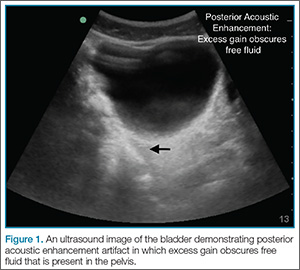
Fanning Is Key
With the probe placed at a single location on the skin, one can dramatically change the structures visualized by fanning (tilting the probe). The image visualized on the ultrasound screen represents only a single slice of the anatomy—one that is about the thickness of a credit card. A single image therefore can only show structures that are within that thin beam of the probe. Just as one would not make a clinical decision based on a single-slice computed tomography (CT) scan image, the same is true of ultrasound. By fanning the probe toward the anterior and posterior abdomen, the clinician will catch smaller quantities of free fluid within each quadrant. A good rule of thumb is to scan through the entire organ of interest from edge-to-edge (eg, the entire bladder when imaging the pelvic window; the entire kidney in the right upper quadrant (RUQ) window; the entire spleen in the left upper quadrant [LUQ]).
Get Rid of the Rib Shadows
The RUQ and LUQ windows can be difficult to visualize when the view is obscured by rib shadows. To minimize/remove rib shadows, some clinicians prefer to use the phased array probe, which has a small footprint that fits easily in the intercostal space. Clinicians who prefer using the curvilinear probe should place the probe at an oblique angle (Figure 2); this probe will fit between the ribs and remove shadowing artifacts.
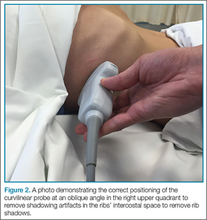
Remember the Paracolic
In some patients, the paracolic gutters are the most dependent portion of the abdomen and the first place where free fluid collects. When evaluating the RUQ, the clinician should first identify Morrison’s pouch, which is the interface between the liver and the kidney. After this pouch has been identified, the clinician should slide the probe toward the patient’s feet, paying close attention to the area around the inferior tip of the liver, and continue sliding the probe down to the inferior tip of the kidney, looking for fluid layering above the kidney or the psoas muscle (Figure 3). The same holds true for the LUQ technique. Once one has looked between the spleen and the diaphragm for free fluid, the probe should be moved down to the flank to evaluate the inferior tip of the spleen and the region anterior to the kidney.
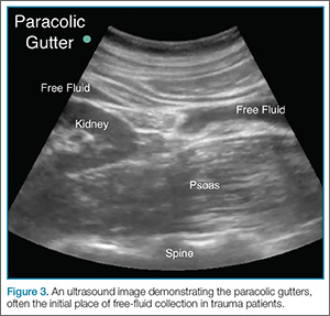
The Left Upper Quadrant—Do Not Let the Stomach Fake You Out
A fluid-filled stomach can be a fake-out for free fluid appearing black on ultrasound (Figure 4). Remember, free fluid in the LUQ window will typically appear between the spleen and the diaphragm or at either pole of the spleen, so the clinician should pay particular attention to these areas. When evaluating the LUQ, a good rule of thumb is to place one’s hand on the patient’s bed while holding the probe; this will ensure that the scan is sufficiently posterior. The probe may also need to be fanned toward the bed to identify the kidneys in the retroperitoneum.
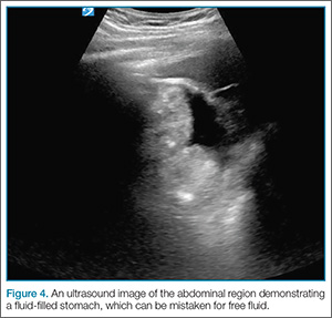
Look in the Chest and Remember the Spine Sign
Rapidly identifying a hemothorax can be a critical finding on the EFAST examination. Therefore, it is important to remember that air in the lungs scatters sound waves, so one does not normally visualize distinct structures that are deep to the pleural line. This is why the spine is not typically visible in the chest above the level of the diaphragm. When pathology is present, however, the sound waves are not blocked by air-filled lungs and one can see the “spine sign,” which suggests the presence of either effusion or consolidation of the lung (Figure 5).
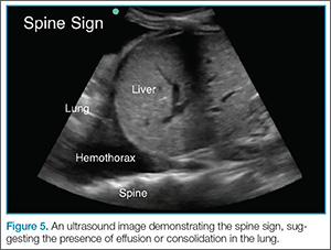
Tough Cardiac Window? Try These Tips
A subxiphoid window is typically used to assess for pericardial effusion. To obtain this view, the clinician usually needs to increase the depth setting by a few centimeters (typically to around 18 cm). When the patient is able to do so, he or she may assist in the examination by bending his or her knees or taking a deep breath to help bring the heart into view. Despite these efforts, however, in some patients, it is technically impossible to obtain a subxiphoid view. In such cases, switching to an alternate view, such as the parasternal window, may be successful in visualizing the subxiphoid region.
Summary
Proper gain adjustment, thorough scanning of the thoracoabdominal region, and knowledge of common artifacts and signs are essential to ensuring an accurate and thorough POC EFAST examination.
The extended focused assessment with sonography for trauma (EFAST) examination provides rapid point-of-care (POC) evaluation of patients with thoracoabdominal trauma. This article offers essential clinical pearls to ensure an accurate and thorough examination, including tips on proper gain adjustment, correct probe fanning, shadow removal, visualization of the paracolic gutters, seeking the “spine sign” to determine effusion, and assessing effusion or consolidation of the lung.
Turning Down the Gain
Too much gain (signal amplification) will wash out the ultrasound image, making it challenging to detect small quantities of free fluid. This is especially true in the pelvic windows. Sound waves travel easily through the fluid-filled bladder and a posterior acoustic enhancement artifact will make the far field of the image appear too bright, obscuring small quantities of fluid (Figure 1). To correct this issue without changing the gain of the entire image, the far-field gain can be adjusted on most ultrasound devices by using the time-gain compensation bar or a far field gain knob.
Fanning Is Key
With the probe placed at a single location on the skin, one can dramatically change the structures visualized by fanning (tilting the probe). The image visualized on the ultrasound screen represents only a single slice of the anatomy—one that is about the thickness of a credit card. A single image therefore can only show structures that are within that thin beam of the probe. Just as one would not make a clinical decision based on a single-slice computed tomography (CT) scan image, the same is true of ultrasound. By fanning the probe toward the anterior and posterior abdomen, the clinician will catch smaller quantities of free fluid within each quadrant. A good rule of thumb is to scan through the entire organ of interest from edge-to-edge (eg, the entire bladder when imaging the pelvic window; the entire kidney in the right upper quadrant (RUQ) window; the entire spleen in the left upper quadrant [LUQ]).
Get Rid of the Rib Shadows
The RUQ and LUQ windows can be difficult to visualize when the view is obscured by rib shadows. To minimize/remove rib shadows, some clinicians prefer to use the phased array probe, which has a small footprint that fits easily in the intercostal space. Clinicians who prefer using the curvilinear probe should place the probe at an oblique angle (Figure 2); this probe will fit between the ribs and remove shadowing artifacts.
Remember the Paracolic
In some patients, the paracolic gutters are the most dependent portion of the abdomen and the first place where free fluid collects. When evaluating the RUQ, the clinician should first identify Morrison’s pouch, which is the interface between the liver and the kidney. After this pouch has been identified, the clinician should slide the probe toward the patient’s feet, paying close attention to the area around the inferior tip of the liver, and continue sliding the probe down to the inferior tip of the kidney, looking for fluid layering above the kidney or the psoas muscle (Figure 3). The same holds true for the LUQ technique. Once one has looked between the spleen and the diaphragm for free fluid, the probe should be moved down to the flank to evaluate the inferior tip of the spleen and the region anterior to the kidney.
The Left Upper Quadrant—Do Not Let the Stomach Fake You Out
A fluid-filled stomach can be a fake-out for free fluid appearing black on ultrasound (Figure 4). Remember, free fluid in the LUQ window will typically appear between the spleen and the diaphragm or at either pole of the spleen, so the clinician should pay particular attention to these areas. When evaluating the LUQ, a good rule of thumb is to place one’s hand on the patient’s bed while holding the probe; this will ensure that the scan is sufficiently posterior. The probe may also need to be fanned toward the bed to identify the kidneys in the retroperitoneum.
Look in the Chest and Remember the Spine Sign
Rapidly identifying a hemothorax can be a critical finding on the EFAST examination. Therefore, it is important to remember that air in the lungs scatters sound waves, so one does not normally visualize distinct structures that are deep to the pleural line. This is why the spine is not typically visible in the chest above the level of the diaphragm. When pathology is present, however, the sound waves are not blocked by air-filled lungs and one can see the “spine sign,” which suggests the presence of either effusion or consolidation of the lung (Figure 5).
Tough Cardiac Window? Try These Tips
A subxiphoid window is typically used to assess for pericardial effusion. To obtain this view, the clinician usually needs to increase the depth setting by a few centimeters (typically to around 18 cm). When the patient is able to do so, he or she may assist in the examination by bending his or her knees or taking a deep breath to help bring the heart into view. Despite these efforts, however, in some patients, it is technically impossible to obtain a subxiphoid view. In such cases, switching to an alternate view, such as the parasternal window, may be successful in visualizing the subxiphoid region.
Summary
Proper gain adjustment, thorough scanning of the thoracoabdominal region, and knowledge of common artifacts and signs are essential to ensuring an accurate and thorough POC EFAST examination.
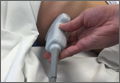
A Guide to Ultrasound of the Shoulder, Part 2: The Diagnostic Evaluation
The musculoskeletal (MSK) ultrasound evaluation of the shoulder provides a cost- and time-efficient imaging modality with similar diagnostic power as magnetic resonance imaging (MRI).1,2 Its portable point-of-care applications can be used in the office, in the operating room, and in sideline athletic event coverage, as we discussed in Part 1 of this series.3
MSK ultrasound may seem difficult and daunting, and many articles have quoted steep learning curves.4,5 However, in our experience in teaching many ultrasound courses, this modality can be learned quite quickly with the proper instruction. Physicians are already familiar with anatomy and usually have had some exposure to MRI.4 Taking courses in MSK ultrasound or simply learning the basic concepts of ultrasound and then learning the machine controls is usually a good start.5-8 Practice scanning normal individuals, comparing the images from an MRI to learn how to reproduce the same planes and images. This will allow the user to become familiar with normal anatomy and how to see the images on the ultrasound screen.5-8 Vollman and colleagues9 showed that in trainees, combining MRI images with sonograms enhances the ability to correctly identify MSK ultrasound anatomy from 40.9% to 72.5%, when compared with learning from ultrasound images alone.
There are currently no certifications necessary to perform ultrasound scans or bill for them; however, some insurance carriers may require demonstrating relevant, documented training for reimbursement.3 Various organizations are trying to develop certifications and regulations for ultrasound to standardize the use of this modality. In the United States, the American Institute of Ultrasound in Medicine (AIUM) and the American Registry for Diagnostic Medical Sonography (ARDMS) provide guidelines and particular MSK ultrasound certifications.10,11
Basic Ultrasound Principles
The ultrasound machine creates electrical impulses that are turned into sound waves by piezoelectric crystals at the probe’s footprint. These sound waves bounce off tissues and return to the probe, where they are converted electronically to an image on the monitor. Depending on the echogenicity of the scanned tissue, the ultrasound beam will either reflect or be absorbed at different rates. This variance is transmitted on the monitor as a grayscale image. When ultrasound waves are highly reflective, like in bone or fat, they are characterized as hyperechoic. The opposite occurs when ultrasound waves are absorbed like in the fluid of a cystic cavity or joint effusion, and the image appears black. This is described as anechoic.12 Intermediate tissues such as tendons that are less reflective are seen as hypoechoic and appear gray. When a tissue has a similar echogenicity to its surrounding tissues, it is called isoechoic.12
The transducer is the scanning component of the ultrasound machine. Transducers come in 2 shapes: linear and curvilinear. The linear probe creates a straight image that is equal to the size of the transducer footprint. The curvilinear probe creates a wider, wedge-shaped panoramic image.
Linear probes are of higher frequency and generate higher resolution images of shallower structures, while curvilinear probes have greater depth penetration but generate lower resolution images. A high frequency of 10 to 15 MHz is preferred for anatomy between 2 cm to 4 cm depth.13 Midrange frequency of 5 to 10 MHz is preferred at 5 cm to 6 cm depth, and low-frequency 2 to 5 MHz probes are preferred for anatomical structures >6 cm depth.13
Anisotropy is the property of being directionally dependent, as opposed to isotropy, which implies identical properties in all directions. This anisotropic effect is dependent on the angle of the insonating beam. The maximum return echo occurs when the ultrasound beam is perpendicular to the tendon. Decreasing the insonating angle on a normal tendon will cause it to change from brightly hyperechoic (the actual echo from tightly bound tendon fibers) to darkly hypoechoic. If the angle is then increased, the tendon will again appear hyperechoic. If the artifact causes a normal tendon to appear hypoechoic, it may falsely lead to a diagnosis of tendinosis or tear.
Posterior acoustic shadowing is present when a hyperechoic structure reflects the ultrasound beam so much that it creates a dark shadow underneath it.12,14 This phenomenon is possible since the ultrasound beam cannot penetrate the hyperechoic structure and reflects off its inferior tissues. Reverberation is when the beam is repeated back and forth between 2 parallel highly reflective surfaces. The initial reflection will be displayed correctly, while the subsequent ultrasound waves will be delayed and appear at a farther distance from the transducer.12,14
The point where the beam is at its narrowest point generates the section of the image that is best visualized.15 This is called the focal zone, and it can be adjusted to highlight the desired area of evaluation. Gain controls adjust the amount of black, gray, and white on the monitor and can be adjusted to focus the desired image.13 Depth settings are fundamental in finding the desired targets. It is recommended to start with a higher depth setting to get an overview and progressively decrease the depth to key in on the desired anatomy.13 Color Doppler can be used to view movement within structures and to identify vessels, synovitis, and neovascularization in tendinopathy.13
Ultrasound of the Shoulder
Patients should be seated, if possible, on a rotating seat. The examiner’s shoulder should be higher than the patient’s shoulder.16 The user holds the ultrasound probe between the thumb and index fingers while resting the hypothenar eminence on the patient to serve as a fulcrum and steadying force. The examination should take 5 to 15 minutes, depending on the examiner’s expertise and the amount of anatomy being scanned.
Examining the body requires knowledge of anatomy. The examination and accuracy are determined by the technician using the probe. The probe can be angled any direction and be placed obliquely on the subject. The advantage here is that anatomy in the human body is not always planar. Muscles and tissues can run obliquely or even perpendicular to each other. When evaluating anatomy, the examiner should keep in mind what structure he or she is looking for; where it should be found; what landmarks can be used to easily locate it; what orientation it has; and what the normal anatomy should look like.
Muscle appears as a lattice with larger areas of hypoechoic muscle tissue and hyperechoic fascial perimysium layers traversing through it.17 The actual muscle tissue appears hypoechoic from the fluid or blood found within. Scarring, fibrosis, calcification, or chronic injury will change the tissue to appear denser or hyperechoic.17 Acute injury will appear hypoechoic from the inflammatory response and influx of blood. Tendon appears dense and hyperechoic with striations within the tissue, sometimes referred to as a horse’s tail.17 When torn, there will be a disassociation of the tissue with a hypoechoic region between the 2 ends. The attachment to the bone and muscle tissue should appear uniform. Hyperechoic areas within the tendon may be from calcification. Ligament appears similar to tendon but is more isoechoic and connects bone to bone. Evaluation of the entire length and the attachments to the bone are critical to evaluate for disease.
Bone appears bright hyperechoic, smooth, and flat, while hyaline cartilage is hypoechoic, smooth, and runs superiorly in a parallel pattern to its respective inferior cortical bone.17
Fibrocartilage is hyperechoic and typically triangularly shaped, such as in the glenohumeral labrum. Nerves appear fascicular and hypoechoic surrounded by hyperechoic epineurium.14
The epidermis and dermis are the most superficial structure on top of the screen, and are also hyperechoic.17
The Diagnostic Shoulder Examination
The proximal long head of the biceps tendon (LHBT) is the easiest structure in the shoulder to identify because of the anatomic structure, the bicipital groove. By keeping the arm relaxed, perpendicular to the ground, and in neutral rotation, the probe can be placed perpendicular to the arm over the proximal shoulder (Figure 1A).16-20 By finding the groove, the biceps tendon will usually be found resting within the groove (Figure 1B). This is the short axis view and is equivalent to an MRI in the axial plane.
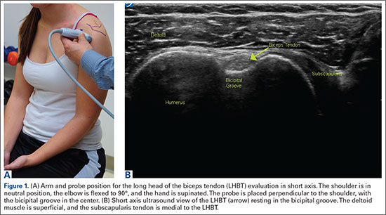
The long axis view of the proximal biceps tendon is found by keeping the tendon in the center of the screen/probe. The probe is then rotated 90° on its center axis, keeping the tendon centered on the probe. The user should be sure to visualize the entire tendon on the screen. If only part of the tendon is seen along only part of the screen, then the probe is oblique to the tendon. In this case, the probe area showing the tendon must be stabilized as the center or set point. The other part of the probe will then pivot until all of the tendon is seen on the screen. The MRI equivalent to the long axis of the proximal biceps tendon is the sagittal view.
Ultrasound is a dynamic evaluation. Moving the probe or moving the patient will change what and how something is imaged. The proximal biceps tendon is a good example of this concept. The bicipital groove is very deep proximally and flattens out as it travels distally to the mid-humerus. The examiner should continually adjust his or her hand/probe/patient position as well as depth/gain and other console functions to adapt to the dynamics of the scan. While keeping the bicep tendon in a short axis view, the tendon can be dynamically evaluated for subluxation by internally and externally rotating the arm.
To find the subscapularis, the arm remains in a neutral position with the hand supinated and the probe is held parallel with the ground. After finding the bicipital groove, the subscapularis tendon insertion is just medial to the groove (Figure 1B). By externally rotating the arm, the subscapularis tendon/muscle will come into a long axis view.16-20 The MRI equivalent to the long axis view of the subscapularis is the axial view. Dynamic testing can be done by internally and externally rotating the arm to evaluate for impingement of the subscapularis tendon as it slides underneath the coracoid process. To view the subscapularis tendon in short axis, the tendon is kept in the center of the screen/probe, and the probe is then rotated 90° on its center axis, keeping the tendon centered on the probe. The MRI equivalent is the sagittal view.
Some have recommended using the modified Crass or Middleton position to evaluate the supraspinatus, where the hand is in the “back pocket”.19 However, many patients with shoulder pain have trouble with this position. By resting the ipsilateral hand on the ipsilateral hip and then dropping the elbow, the supraspinatus insertion can still be brought out from under the acromion. This does bring the insertion anterior out of the scapular plane, so an adjustment is required in probe positioning to properly see the supraspinatus short and long axis. To find the long axis, the probe is placed parallel to a plane that spans the contralateral shoulder and ipsilateral hip (Figure 2A). The fibers of the supraspinatus should be inserting directly lateral to the humeral head without any intervening space (Figure 2B). If any space exists, a partial articular supraspinatus tendon avulsion (PASTA) lesion is present, and its thickness can be directly measured. Moving more posterior will show the flattening of the tuberosity and the fibers of the infraspinatus moving away from the humeral head—the bare spot. The MRI equivalent is the coronal view.
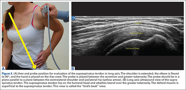
To view the supraspinatus tendon in short axis, maintain the arm in the same position, keeping the tendon in the center of the screen/probe. The probe is then rotated 90° on its center axis, keeping the tendon centered on the probe. The probe should now be in a parallel plane between the ipsilateral shoulder and the contralateral hip. The biceps tendon in cross-section will be found anteriorly, and the articular cartilage will appear as a black layer over the bone. Dynamic testing includes placing the probe in a coronal plane between the acromion and greater tuberosity. When the patient abducts the arm while in internal rotation, the supraspinatus tendon will slide underneath the coracoacromial arch showing potential external impingement.15 The MRI equivalent is the sagittal plane.
The glenohumeral joint is best viewed posteriorly, limiting how much of the intra-articular portion of the joint can be imaged. The arm remains in a neutral position; palpate for the posterior acromion and place the probe just inferior to it, wedging up against it (Figure 3A). The glenohumeral joint will be seen by keeping the probe parallel to the ground (Figure 3B). The MRI equivalent is the axial plane. If a joint effusion exists, it can be seen in the posterior recess.15 A hyperechoic triangular region in between the humeral head and the glenoid will represent the glenoid labrum (Figure 3B). By internally and externally rotating the arm, the joint and labrum complex can be dynamically examined. From the labrum, scanning superior and medial can sometimes show the spinoglenoid notch where a paralabral cyst might be seen.15
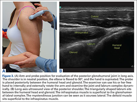
Using the glenohumeral joint as a reference, the infraspinatus muscle is easily visualized. Maintaining the arm in neutral position with the probe over the glenohumeral joint, the infraspinatus will become apparent as it lays in long axis view superficially between the posterior deltoid and glenohumeral joint (Figure 3B).16-20 The teres minor lies just inferiorly. The MRI equivalent is the axial plane. To view the infraspinatus and teres minor in short axis, the probe is then rotated 90° on its center axis. The infraspinatus (superiorly) and teres minor (inferiorly) muscles will be visible in short axis within the infraspinatus fossa.15 The MRI equivalent is the sagittal view.
The acromioclavicular joint is superficial and easy to image. The arm remains in a neutral position, and we can palpate the joint for easy localization. The probe is placed anteriorly in a coronal plane over the acromion and clavicle. By scanning anteriorly and posteriorly, a joint effusion referred to as a Geyser sign might be seen. The MRI equivalent is the coronal view.
Available Certifications
The AIUM certification is a voluntary peer reviewed process that acknowledges that a practice is meeting national standards and aids in improving their respective MSK ultrasound protocols. They also provide guidelines on demonstrating training and competence on performing and/or interpreting diagnostic MSK examinations (Table).10 The ARDMS certification provides an actual individual certification referred to as “Registered” in MSK ultrasound.11 The physician must perform 150 diagnostic MSK ultrasound evaluations within 36 months of applying and pass a 200-question examination that is offered twice per year.11 None of these certifications are mandated by the American Medical Association (AMA) or American Osteopathic Association (AOA).
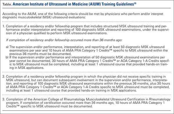
Maintenance and Continuing Medical Education (CME)
The AIUM recommends that a minimum of 50 diagnostic MSK ultrasound evaluations be performed per year for skill maintenance.10 Furthermore, 10 hours of AMA PRA Category 1 Credits™ or American Osteopathic Association Category 1-A Credits specific to MSK ultrasound must be completed by physicians performing and/or interpreting these examinations every 3 years.10 ARDMS recommends a minimum of 30 MSK ultrasound-specific CMEs in preparation for their “Registered” MSK evaluation.1
Conclusion
MSK ultrasound is a dynamic, real-time imaging modality that can improve cost efficiency and patient care. Its portability allows for its use anywhere. Learning the skill may seem daunting, but with the proper courses and education, the technology can be easily learned. By correlating a known modality like MRI, the user will easily begin to read ultrasound images. No current certification is needed to use or bill for ultrasound, but various institutions are developing criteria and testing. Two organizations, AIUM and ARDMS, provide guidelines and certifications to demonstrate competency, which may become necessary in the very near future.
1. Sivan M, Brown J, Brennan S, Bhakta B. A one-stop approach to the management of soft tissue and degenerative musculoskeletal conditions using clinic-based ultrasonography. Musculoskeletal Care. 2011;9(2):63-68.
2. Roy J-S, Braën C, Leblond J, et al. Diagnostic accuracy of ultrasonography, MRI and MR arthrography in the characterization of rotator cuff disorders: a meta-analysis [published online ahead of print February 11, 2015]. Br J Sports Med. doi:10.1136/bjsports-2014-094148.
3. Hirahara AM, Panero AJ. A guide to ultrasound of the shoulder, part 1: coding and reimbursement. Am J Orthop. 2016;45(3):176-182.
4. Hama M, Takase K, Ihata A, et al. Challenges to expanding the clinical application of musculoskeletal ultrasonography (MSUS) among rheumatologists: from a second survey in Japan. Mod Rheumatol. 2012;2:202-208.
5. Smith MJ, Rogers A, Amso N, Kennedy J, Hall A, Mullaney P. A training, assessment and feedback package for the trainee shoulder sonographer. Ultrasound. 2015;23(1):29-41.
6. Delzell PB, Boyle A, Schneider E. Dedicated training program for shoulder sonography: the results of a quality program reverberate with everyone. J Ultrasound Med. 2015;34(6):1037-1042.
7. Finnoff JT, Berkoff D, Brennan F, et al. American Medical Society for Sports Medicine (AMSSM) recommended sports ultrasound curriculum for sports medicine fellowships. PM R. 2015;7(2)e1-e11.
8. Adelman S, Fishman P. Use of portable ultrasound machine for outpatient orthopedic diagnosis: an implementation study. Perm J. 2013;17(3):18-22.
9. Vollman A, Hulen R, Dulchavsky S, et al. Educational benefits of fusing magnetic resonance imaging with sonograms. J Clin Ultrasound. 2014;42(5) 257-263.
10. Training guidelines for physicians and chiropractors who evaluate and interpret diagnostic musculoskeletal ultrasound examinations. Laurel, MD: American Institute of Ultrasound in Medicine; 2014. http://www.aium.org/resources/viewStatement.aspx?id=51. Accessed February 26, 2016.
11. Registered in musculoskeletal (RMSK) sonography. American Registry for Diagnostic Medical Sonography Web site. http://www.ardms.org/get-certified/RMSK/Pages/RMSK.aspx. Accessed February 26, 2016.
12. Silkowski C. Ultrasound nomenclature, image orientation, and basic instrumentation. In: Abraham D, Silkowski C, Odwin C, eds. Emergency Medicine Sonography Pocket Guide to Sonographic Anatomy and Pathology. Sudbury, MA: Jones and Bartlett; 2010:1-24.
13. Ihnatsenka B, Boezaart AP. Ultrasound: basic understanding and learning the language. Int J Shoulder Surg. 2010;4(3):55-62.
14. Taljanovic MS, Melville DM, Scalcione LR, Gimber LH, Lorenz EJ, Witte RS. Artifacts in musculoskeletal ultrasonography. Semin Musculoskelet Radiol. 2014;18(1):3-11.
15. Ng A, Swanevelder J. Resolution in ultrasound imaging. Continuing Educ Anaesth Crit Care Pain. 2011;11(5):186-192. http://ceaccp.oxfordjournals.org/content/11/5/186.full. Accessed March 3, 2016.
16. Nazarian L, Bohm-Velez M, Kan JH, et al. AIUM practice parameters for the performance of a musculoskeletal ultrasound examination. Laurel, MD: American Institute of Ultrasound in Medicine; 2012. http://www.aium.org/resources/guidelines/musculoskeletal.pdf. Accessed February 26, 2016.
17. Jacobson J. Fundamentals of Musculoskeletal Ultrasound. 2nd edition. Philadelphia, PA: Elsevier Saunders; 2013.
18. The Ultrasound Subcommittee of the European Society of Musculoskeletal Radiology. Musculoskeletal ultrasound: technique guidelines. Insights Imaging. 2010;1:99-141.
19. Corazza A, Orlandi D, Fabbro E, et al. Dynamic high-resolution ultrasound of the shoulder: how we do it. Eur J Radiol. 2015;84(2):266-277.
20. Allen GM. Shoulder ultrasound imaging-integrating anatomy, biomechanics and disease processes. Eur J Radiol. 2008;68(1):137-146
The musculoskeletal (MSK) ultrasound evaluation of the shoulder provides a cost- and time-efficient imaging modality with similar diagnostic power as magnetic resonance imaging (MRI).1,2 Its portable point-of-care applications can be used in the office, in the operating room, and in sideline athletic event coverage, as we discussed in Part 1 of this series.3
MSK ultrasound may seem difficult and daunting, and many articles have quoted steep learning curves.4,5 However, in our experience in teaching many ultrasound courses, this modality can be learned quite quickly with the proper instruction. Physicians are already familiar with anatomy and usually have had some exposure to MRI.4 Taking courses in MSK ultrasound or simply learning the basic concepts of ultrasound and then learning the machine controls is usually a good start.5-8 Practice scanning normal individuals, comparing the images from an MRI to learn how to reproduce the same planes and images. This will allow the user to become familiar with normal anatomy and how to see the images on the ultrasound screen.5-8 Vollman and colleagues9 showed that in trainees, combining MRI images with sonograms enhances the ability to correctly identify MSK ultrasound anatomy from 40.9% to 72.5%, when compared with learning from ultrasound images alone.
There are currently no certifications necessary to perform ultrasound scans or bill for them; however, some insurance carriers may require demonstrating relevant, documented training for reimbursement.3 Various organizations are trying to develop certifications and regulations for ultrasound to standardize the use of this modality. In the United States, the American Institute of Ultrasound in Medicine (AIUM) and the American Registry for Diagnostic Medical Sonography (ARDMS) provide guidelines and particular MSK ultrasound certifications.10,11
Basic Ultrasound Principles
The ultrasound machine creates electrical impulses that are turned into sound waves by piezoelectric crystals at the probe’s footprint. These sound waves bounce off tissues and return to the probe, where they are converted electronically to an image on the monitor. Depending on the echogenicity of the scanned tissue, the ultrasound beam will either reflect or be absorbed at different rates. This variance is transmitted on the monitor as a grayscale image. When ultrasound waves are highly reflective, like in bone or fat, they are characterized as hyperechoic. The opposite occurs when ultrasound waves are absorbed like in the fluid of a cystic cavity or joint effusion, and the image appears black. This is described as anechoic.12 Intermediate tissues such as tendons that are less reflective are seen as hypoechoic and appear gray. When a tissue has a similar echogenicity to its surrounding tissues, it is called isoechoic.12
The transducer is the scanning component of the ultrasound machine. Transducers come in 2 shapes: linear and curvilinear. The linear probe creates a straight image that is equal to the size of the transducer footprint. The curvilinear probe creates a wider, wedge-shaped panoramic image.
Linear probes are of higher frequency and generate higher resolution images of shallower structures, while curvilinear probes have greater depth penetration but generate lower resolution images. A high frequency of 10 to 15 MHz is preferred for anatomy between 2 cm to 4 cm depth.13 Midrange frequency of 5 to 10 MHz is preferred at 5 cm to 6 cm depth, and low-frequency 2 to 5 MHz probes are preferred for anatomical structures >6 cm depth.13
Anisotropy is the property of being directionally dependent, as opposed to isotropy, which implies identical properties in all directions. This anisotropic effect is dependent on the angle of the insonating beam. The maximum return echo occurs when the ultrasound beam is perpendicular to the tendon. Decreasing the insonating angle on a normal tendon will cause it to change from brightly hyperechoic (the actual echo from tightly bound tendon fibers) to darkly hypoechoic. If the angle is then increased, the tendon will again appear hyperechoic. If the artifact causes a normal tendon to appear hypoechoic, it may falsely lead to a diagnosis of tendinosis or tear.
Posterior acoustic shadowing is present when a hyperechoic structure reflects the ultrasound beam so much that it creates a dark shadow underneath it.12,14 This phenomenon is possible since the ultrasound beam cannot penetrate the hyperechoic structure and reflects off its inferior tissues. Reverberation is when the beam is repeated back and forth between 2 parallel highly reflective surfaces. The initial reflection will be displayed correctly, while the subsequent ultrasound waves will be delayed and appear at a farther distance from the transducer.12,14
The point where the beam is at its narrowest point generates the section of the image that is best visualized.15 This is called the focal zone, and it can be adjusted to highlight the desired area of evaluation. Gain controls adjust the amount of black, gray, and white on the monitor and can be adjusted to focus the desired image.13 Depth settings are fundamental in finding the desired targets. It is recommended to start with a higher depth setting to get an overview and progressively decrease the depth to key in on the desired anatomy.13 Color Doppler can be used to view movement within structures and to identify vessels, synovitis, and neovascularization in tendinopathy.13
Ultrasound of the Shoulder
Patients should be seated, if possible, on a rotating seat. The examiner’s shoulder should be higher than the patient’s shoulder.16 The user holds the ultrasound probe between the thumb and index fingers while resting the hypothenar eminence on the patient to serve as a fulcrum and steadying force. The examination should take 5 to 15 minutes, depending on the examiner’s expertise and the amount of anatomy being scanned.
Examining the body requires knowledge of anatomy. The examination and accuracy are determined by the technician using the probe. The probe can be angled any direction and be placed obliquely on the subject. The advantage here is that anatomy in the human body is not always planar. Muscles and tissues can run obliquely or even perpendicular to each other. When evaluating anatomy, the examiner should keep in mind what structure he or she is looking for; where it should be found; what landmarks can be used to easily locate it; what orientation it has; and what the normal anatomy should look like.
Muscle appears as a lattice with larger areas of hypoechoic muscle tissue and hyperechoic fascial perimysium layers traversing through it.17 The actual muscle tissue appears hypoechoic from the fluid or blood found within. Scarring, fibrosis, calcification, or chronic injury will change the tissue to appear denser or hyperechoic.17 Acute injury will appear hypoechoic from the inflammatory response and influx of blood. Tendon appears dense and hyperechoic with striations within the tissue, sometimes referred to as a horse’s tail.17 When torn, there will be a disassociation of the tissue with a hypoechoic region between the 2 ends. The attachment to the bone and muscle tissue should appear uniform. Hyperechoic areas within the tendon may be from calcification. Ligament appears similar to tendon but is more isoechoic and connects bone to bone. Evaluation of the entire length and the attachments to the bone are critical to evaluate for disease.
Bone appears bright hyperechoic, smooth, and flat, while hyaline cartilage is hypoechoic, smooth, and runs superiorly in a parallel pattern to its respective inferior cortical bone.17
Fibrocartilage is hyperechoic and typically triangularly shaped, such as in the glenohumeral labrum. Nerves appear fascicular and hypoechoic surrounded by hyperechoic epineurium.14
The epidermis and dermis are the most superficial structure on top of the screen, and are also hyperechoic.17
The Diagnostic Shoulder Examination
The proximal long head of the biceps tendon (LHBT) is the easiest structure in the shoulder to identify because of the anatomic structure, the bicipital groove. By keeping the arm relaxed, perpendicular to the ground, and in neutral rotation, the probe can be placed perpendicular to the arm over the proximal shoulder (Figure 1A).16-20 By finding the groove, the biceps tendon will usually be found resting within the groove (Figure 1B). This is the short axis view and is equivalent to an MRI in the axial plane.
The long axis view of the proximal biceps tendon is found by keeping the tendon in the center of the screen/probe. The probe is then rotated 90° on its center axis, keeping the tendon centered on the probe. The user should be sure to visualize the entire tendon on the screen. If only part of the tendon is seen along only part of the screen, then the probe is oblique to the tendon. In this case, the probe area showing the tendon must be stabilized as the center or set point. The other part of the probe will then pivot until all of the tendon is seen on the screen. The MRI equivalent to the long axis of the proximal biceps tendon is the sagittal view.
Ultrasound is a dynamic evaluation. Moving the probe or moving the patient will change what and how something is imaged. The proximal biceps tendon is a good example of this concept. The bicipital groove is very deep proximally and flattens out as it travels distally to the mid-humerus. The examiner should continually adjust his or her hand/probe/patient position as well as depth/gain and other console functions to adapt to the dynamics of the scan. While keeping the bicep tendon in a short axis view, the tendon can be dynamically evaluated for subluxation by internally and externally rotating the arm.
To find the subscapularis, the arm remains in a neutral position with the hand supinated and the probe is held parallel with the ground. After finding the bicipital groove, the subscapularis tendon insertion is just medial to the groove (Figure 1B). By externally rotating the arm, the subscapularis tendon/muscle will come into a long axis view.16-20 The MRI equivalent to the long axis view of the subscapularis is the axial view. Dynamic testing can be done by internally and externally rotating the arm to evaluate for impingement of the subscapularis tendon as it slides underneath the coracoid process. To view the subscapularis tendon in short axis, the tendon is kept in the center of the screen/probe, and the probe is then rotated 90° on its center axis, keeping the tendon centered on the probe. The MRI equivalent is the sagittal view.
Some have recommended using the modified Crass or Middleton position to evaluate the supraspinatus, where the hand is in the “back pocket”.19 However, many patients with shoulder pain have trouble with this position. By resting the ipsilateral hand on the ipsilateral hip and then dropping the elbow, the supraspinatus insertion can still be brought out from under the acromion. This does bring the insertion anterior out of the scapular plane, so an adjustment is required in probe positioning to properly see the supraspinatus short and long axis. To find the long axis, the probe is placed parallel to a plane that spans the contralateral shoulder and ipsilateral hip (Figure 2A). The fibers of the supraspinatus should be inserting directly lateral to the humeral head without any intervening space (Figure 2B). If any space exists, a partial articular supraspinatus tendon avulsion (PASTA) lesion is present, and its thickness can be directly measured. Moving more posterior will show the flattening of the tuberosity and the fibers of the infraspinatus moving away from the humeral head—the bare spot. The MRI equivalent is the coronal view.
To view the supraspinatus tendon in short axis, maintain the arm in the same position, keeping the tendon in the center of the screen/probe. The probe is then rotated 90° on its center axis, keeping the tendon centered on the probe. The probe should now be in a parallel plane between the ipsilateral shoulder and the contralateral hip. The biceps tendon in cross-section will be found anteriorly, and the articular cartilage will appear as a black layer over the bone. Dynamic testing includes placing the probe in a coronal plane between the acromion and greater tuberosity. When the patient abducts the arm while in internal rotation, the supraspinatus tendon will slide underneath the coracoacromial arch showing potential external impingement.15 The MRI equivalent is the sagittal plane.
The glenohumeral joint is best viewed posteriorly, limiting how much of the intra-articular portion of the joint can be imaged. The arm remains in a neutral position; palpate for the posterior acromion and place the probe just inferior to it, wedging up against it (Figure 3A). The glenohumeral joint will be seen by keeping the probe parallel to the ground (Figure 3B). The MRI equivalent is the axial plane. If a joint effusion exists, it can be seen in the posterior recess.15 A hyperechoic triangular region in between the humeral head and the glenoid will represent the glenoid labrum (Figure 3B). By internally and externally rotating the arm, the joint and labrum complex can be dynamically examined. From the labrum, scanning superior and medial can sometimes show the spinoglenoid notch where a paralabral cyst might be seen.15
Using the glenohumeral joint as a reference, the infraspinatus muscle is easily visualized. Maintaining the arm in neutral position with the probe over the glenohumeral joint, the infraspinatus will become apparent as it lays in long axis view superficially between the posterior deltoid and glenohumeral joint (Figure 3B).16-20 The teres minor lies just inferiorly. The MRI equivalent is the axial plane. To view the infraspinatus and teres minor in short axis, the probe is then rotated 90° on its center axis. The infraspinatus (superiorly) and teres minor (inferiorly) muscles will be visible in short axis within the infraspinatus fossa.15 The MRI equivalent is the sagittal view.
The acromioclavicular joint is superficial and easy to image. The arm remains in a neutral position, and we can palpate the joint for easy localization. The probe is placed anteriorly in a coronal plane over the acromion and clavicle. By scanning anteriorly and posteriorly, a joint effusion referred to as a Geyser sign might be seen. The MRI equivalent is the coronal view.
Available Certifications
The AIUM certification is a voluntary peer reviewed process that acknowledges that a practice is meeting national standards and aids in improving their respective MSK ultrasound protocols. They also provide guidelines on demonstrating training and competence on performing and/or interpreting diagnostic MSK examinations (Table).10 The ARDMS certification provides an actual individual certification referred to as “Registered” in MSK ultrasound.11 The physician must perform 150 diagnostic MSK ultrasound evaluations within 36 months of applying and pass a 200-question examination that is offered twice per year.11 None of these certifications are mandated by the American Medical Association (AMA) or American Osteopathic Association (AOA).
Maintenance and Continuing Medical Education (CME)
The AIUM recommends that a minimum of 50 diagnostic MSK ultrasound evaluations be performed per year for skill maintenance.10 Furthermore, 10 hours of AMA PRA Category 1 Credits™ or American Osteopathic Association Category 1-A Credits specific to MSK ultrasound must be completed by physicians performing and/or interpreting these examinations every 3 years.10 ARDMS recommends a minimum of 30 MSK ultrasound-specific CMEs in preparation for their “Registered” MSK evaluation.1
Conclusion
MSK ultrasound is a dynamic, real-time imaging modality that can improve cost efficiency and patient care. Its portability allows for its use anywhere. Learning the skill may seem daunting, but with the proper courses and education, the technology can be easily learned. By correlating a known modality like MRI, the user will easily begin to read ultrasound images. No current certification is needed to use or bill for ultrasound, but various institutions are developing criteria and testing. Two organizations, AIUM and ARDMS, provide guidelines and certifications to demonstrate competency, which may become necessary in the very near future.
1. Sivan M, Brown J, Brennan S, Bhakta B. A one-stop approach to the management of soft tissue and degenerative musculoskeletal conditions using clinic-based ultrasonography. Musculoskeletal Care. 2011;9(2):63-68.
2. Roy J-S, Braën C, Leblond J, et al. Diagnostic accuracy of ultrasonography, MRI and MR arthrography in the characterization of rotator cuff disorders: a meta-analysis [published online ahead of print February 11, 2015]. Br J Sports Med. doi:10.1136/bjsports-2014-094148.
3. Hirahara AM, Panero AJ. A guide to ultrasound of the shoulder, part 1: coding and reimbursement. Am J Orthop. 2016;45(3):176-182.
4. Hama M, Takase K, Ihata A, et al. Challenges to expanding the clinical application of musculoskeletal ultrasonography (MSUS) among rheumatologists: from a second survey in Japan. Mod Rheumatol. 2012;2:202-208.
5. Smith MJ, Rogers A, Amso N, Kennedy J, Hall A, Mullaney P. A training, assessment and feedback package for the trainee shoulder sonographer. Ultrasound. 2015;23(1):29-41.
6. Delzell PB, Boyle A, Schneider E. Dedicated training program for shoulder sonography: the results of a quality program reverberate with everyone. J Ultrasound Med. 2015;34(6):1037-1042.
7. Finnoff JT, Berkoff D, Brennan F, et al. American Medical Society for Sports Medicine (AMSSM) recommended sports ultrasound curriculum for sports medicine fellowships. PM R. 2015;7(2)e1-e11.
8. Adelman S, Fishman P. Use of portable ultrasound machine for outpatient orthopedic diagnosis: an implementation study. Perm J. 2013;17(3):18-22.
9. Vollman A, Hulen R, Dulchavsky S, et al. Educational benefits of fusing magnetic resonance imaging with sonograms. J Clin Ultrasound. 2014;42(5) 257-263.
10. Training guidelines for physicians and chiropractors who evaluate and interpret diagnostic musculoskeletal ultrasound examinations. Laurel, MD: American Institute of Ultrasound in Medicine; 2014. http://www.aium.org/resources/viewStatement.aspx?id=51. Accessed February 26, 2016.
11. Registered in musculoskeletal (RMSK) sonography. American Registry for Diagnostic Medical Sonography Web site. http://www.ardms.org/get-certified/RMSK/Pages/RMSK.aspx. Accessed February 26, 2016.
12. Silkowski C. Ultrasound nomenclature, image orientation, and basic instrumentation. In: Abraham D, Silkowski C, Odwin C, eds. Emergency Medicine Sonography Pocket Guide to Sonographic Anatomy and Pathology. Sudbury, MA: Jones and Bartlett; 2010:1-24.
13. Ihnatsenka B, Boezaart AP. Ultrasound: basic understanding and learning the language. Int J Shoulder Surg. 2010;4(3):55-62.
14. Taljanovic MS, Melville DM, Scalcione LR, Gimber LH, Lorenz EJ, Witte RS. Artifacts in musculoskeletal ultrasonography. Semin Musculoskelet Radiol. 2014;18(1):3-11.
15. Ng A, Swanevelder J. Resolution in ultrasound imaging. Continuing Educ Anaesth Crit Care Pain. 2011;11(5):186-192. http://ceaccp.oxfordjournals.org/content/11/5/186.full. Accessed March 3, 2016.
16. Nazarian L, Bohm-Velez M, Kan JH, et al. AIUM practice parameters for the performance of a musculoskeletal ultrasound examination. Laurel, MD: American Institute of Ultrasound in Medicine; 2012. http://www.aium.org/resources/guidelines/musculoskeletal.pdf. Accessed February 26, 2016.
17. Jacobson J. Fundamentals of Musculoskeletal Ultrasound. 2nd edition. Philadelphia, PA: Elsevier Saunders; 2013.
18. The Ultrasound Subcommittee of the European Society of Musculoskeletal Radiology. Musculoskeletal ultrasound: technique guidelines. Insights Imaging. 2010;1:99-141.
19. Corazza A, Orlandi D, Fabbro E, et al. Dynamic high-resolution ultrasound of the shoulder: how we do it. Eur J Radiol. 2015;84(2):266-277.
20. Allen GM. Shoulder ultrasound imaging-integrating anatomy, biomechanics and disease processes. Eur J Radiol. 2008;68(1):137-146