User login
Can low-dose aspirin reduce the risk of spontaneous preterm birth?
Antiplatelet agents (mainly low-dose aspirin) have been shown to reduce the risk of preeclampsia in women at risk for the condition. The American College of Obstetricians and Gynecologists currently supports consideration of the use of low-dose aspirin (81 mg/day), initiated between 12 and 28 weeks of gestation, for the prevention of preeclampsia in women at high risk.1
Can antiplatelet agents also reduce the risk of preterm birth? It is a reasonable question, postulate van Vliet and colleagues2: Women with a history of preeclampsia also have an increased risk of spontaneous preterm birth (SPB), and vice versa. Uteroplacental ischemia is present in cases of preeclampsia, and research is showing that uteroplacental ischemia also plays a role in the etiology of spontaneous preterm labor.3,4
Details of the study
To investigate their research question, van Vliet and colleagues performed an additional analysis of the Perinatal Antiplatelet Review of International Studies Individual Participant Data meta-analysis. The original meta-analysis involved the data of 32,217 women at risk for preeclampsia who were randomly assigned to low-dose aspirin-dipyridamole or placebo (no treatment); the study revealed a moderate risk reduction for preeclampsia as well as a significant reduction in preterm birth at less than 34 weeks of gestation in women treated with antiplatelets.2
In the additional analysis, for women with an SPB who began antiplatelet treatment before 20 weeks of gestation, the researchers assessed the time between 20 weeks and spontaneous preterm delivery, iatrogenic preterm delivery, and any preterm delivery. Overall, 9.7% of women (n = 2,670) had an SPB before 37 weeks of gestation, 2.8% (n = 773) had an SPB before 34 weeks of gestation, and 0.5% (n = 151) had an SPB before 28 weeks of gestation. Antiplatelet agents were associated with a significant reduction in the risk of SPB before 37 weeks (relative risk [RR], 0.93; 95% confidence interval [CI], 0.86–0.996) and before 34 weeks (RR, 0.86; 95% CI, 0.76–0.99). The RR of having an SPB at less than 37 weeks of gestation was 0.83 for women with a previous pregnancy and 0.98 for women in their first pregnancy.2
Bottom line
Antiplatelet use resulted in a 7% reduction in SPB risk in women at risk for preeclampsia. Antiplatelet use resulted in a 14% reduction in moderate to very preterm birth risk (<34 weeks’ gestation).
The authors advise that their study “provides clinicians with the best available evidence to counsel women regarding who might benefit from” antiplatelet use during pregnancy and suggest that antiplatelet use may be a promising intervention for women at high risk for SPB, especially in high-risk women with a previous pregnancy.2
Caveats
The researchers found no difference among those receiving and not receiving antiplatelets in the incidence of antepartum hemorrhage (RR, 1.02; 95% CI, 0.90–1.15), placental abruption (RR, 1.13; 95% CI, 0.87–1.48), or neonatal bleeding (RR, 0.93; 95% CI, 0.80–1.09). The incidence of postpartum hemorrhage (PPH) was again found to be borderline significant (RR, 1.06; 95% CI, 1.00–1.13), but it was more frequent. The authors caution that the SPB reduction that they found in their study (as well as the reduced risk for preeclampsia with low-dose aspirin use) be balanced against the potential higher risk for PPH.2
- The American College of Obstetricians and Gynecologists. Practice advisory on low-dose aspirin and prevention of preeclampsia: updated recommendations. https://www.acog.org/About-ACOG/News-Room/Practice-Advisories/Practice-Advisory-Low-Dose-Aspirin-and-Prevention-of-Preeclampsia-Updated-Recommendations. Updated July 11, 2016. Accessed August 14, 2017.
- van Vliet EO, Askie LA, Mol BW, Oudijk MA. Antiplatelet agents and the prevention of spontaneous preterm birth. Obstet Gynecol. 2017;129(2):327–336.
- Arias F, Rodriquez L, Rayne SC, Kraus FT. Maternal placental vasculopathy and infection: two distinct subgroups among patients with preterm labor and preterm ruptured membranes. Am J Obstet Gynecol. 1993;168(2):585–591.
- Kelly R, Holzman C, Senagore P, et al. Placental vascular pathology findings and pathways of preterm delivery. Am J Epidemiol. 2009;170(2):148–158.
Antiplatelet agents (mainly low-dose aspirin) have been shown to reduce the risk of preeclampsia in women at risk for the condition. The American College of Obstetricians and Gynecologists currently supports consideration of the use of low-dose aspirin (81 mg/day), initiated between 12 and 28 weeks of gestation, for the prevention of preeclampsia in women at high risk.1
Can antiplatelet agents also reduce the risk of preterm birth? It is a reasonable question, postulate van Vliet and colleagues2: Women with a history of preeclampsia also have an increased risk of spontaneous preterm birth (SPB), and vice versa. Uteroplacental ischemia is present in cases of preeclampsia, and research is showing that uteroplacental ischemia also plays a role in the etiology of spontaneous preterm labor.3,4
Details of the study
To investigate their research question, van Vliet and colleagues performed an additional analysis of the Perinatal Antiplatelet Review of International Studies Individual Participant Data meta-analysis. The original meta-analysis involved the data of 32,217 women at risk for preeclampsia who were randomly assigned to low-dose aspirin-dipyridamole or placebo (no treatment); the study revealed a moderate risk reduction for preeclampsia as well as a significant reduction in preterm birth at less than 34 weeks of gestation in women treated with antiplatelets.2
In the additional analysis, for women with an SPB who began antiplatelet treatment before 20 weeks of gestation, the researchers assessed the time between 20 weeks and spontaneous preterm delivery, iatrogenic preterm delivery, and any preterm delivery. Overall, 9.7% of women (n = 2,670) had an SPB before 37 weeks of gestation, 2.8% (n = 773) had an SPB before 34 weeks of gestation, and 0.5% (n = 151) had an SPB before 28 weeks of gestation. Antiplatelet agents were associated with a significant reduction in the risk of SPB before 37 weeks (relative risk [RR], 0.93; 95% confidence interval [CI], 0.86–0.996) and before 34 weeks (RR, 0.86; 95% CI, 0.76–0.99). The RR of having an SPB at less than 37 weeks of gestation was 0.83 for women with a previous pregnancy and 0.98 for women in their first pregnancy.2
Bottom line
Antiplatelet use resulted in a 7% reduction in SPB risk in women at risk for preeclampsia. Antiplatelet use resulted in a 14% reduction in moderate to very preterm birth risk (<34 weeks’ gestation).
The authors advise that their study “provides clinicians with the best available evidence to counsel women regarding who might benefit from” antiplatelet use during pregnancy and suggest that antiplatelet use may be a promising intervention for women at high risk for SPB, especially in high-risk women with a previous pregnancy.2
Caveats
The researchers found no difference among those receiving and not receiving antiplatelets in the incidence of antepartum hemorrhage (RR, 1.02; 95% CI, 0.90–1.15), placental abruption (RR, 1.13; 95% CI, 0.87–1.48), or neonatal bleeding (RR, 0.93; 95% CI, 0.80–1.09). The incidence of postpartum hemorrhage (PPH) was again found to be borderline significant (RR, 1.06; 95% CI, 1.00–1.13), but it was more frequent. The authors caution that the SPB reduction that they found in their study (as well as the reduced risk for preeclampsia with low-dose aspirin use) be balanced against the potential higher risk for PPH.2
- The American College of Obstetricians and Gynecologists. Practice advisory on low-dose aspirin and prevention of preeclampsia: updated recommendations. https://www.acog.org/About-ACOG/News-Room/Practice-Advisories/Practice-Advisory-Low-Dose-Aspirin-and-Prevention-of-Preeclampsia-Updated-Recommendations. Updated July 11, 2016. Accessed August 14, 2017.
- van Vliet EO, Askie LA, Mol BW, Oudijk MA. Antiplatelet agents and the prevention of spontaneous preterm birth. Obstet Gynecol. 2017;129(2):327–336.
- Arias F, Rodriquez L, Rayne SC, Kraus FT. Maternal placental vasculopathy and infection: two distinct subgroups among patients with preterm labor and preterm ruptured membranes. Am J Obstet Gynecol. 1993;168(2):585–591.
- Kelly R, Holzman C, Senagore P, et al. Placental vascular pathology findings and pathways of preterm delivery. Am J Epidemiol. 2009;170(2):148–158.
Marijuana use triples risk of death from hypertension
The risk of death from hypertension is three times greater in adults who use marijuana, compared with nonusers, based on data from a retrospective study of 1,213 adults.
Changes in the legalization of marijuana may promote increased recreational use, but data on the long-term effects of marijuana use on cardiovascular and cerebrovascular mortality are limited, wrote Barbara A. Yankey, PhD, of Georgia State University, Atlanta, and her colleagues.

Data on 686 users and 527 nonusers were combined with the 2011 mortality data from the National Center for Health Statistics (Eur J Prev Cardiol. 2017 Aug 9; doi: 10.1177/2047487317723212).
Overall, marijuana users had a 3.42 times greater risk of death from hypertension than did nonusers (95% confidence interval, 1.20-9.79), and the risk increased by 1.04 for each year of use (95% CI, 1.00-1.07). The average duration of marijuana use was 11.5 years. At the time of study entry, the average age of the participants was 38 years, and the average body mass index was 29 kg/m2; 23% of marijuana users and 21% of nonusers had a prior diagnosis of hypertension.
Of the study participants, 20% used marijuana and smoked cigarettes, 16% used marijuana and were past smokers, 5% were past smokers, and 4% only smoked cigarettes. “In our study, increase in risk for hypertension, [heart disease], or cerebrovascular disease mortality associated with cigarette use was not significant,” the researchers wrote. They attributed this factor to the small sample size and noted that the dangers of cigarette smoking to the cardiovascular system are well established.
The study findings were limited by the relatively small sample size and potentially inaccurate data on the duration of marijuana use, the researchers said.
However, the results suggest that “cardiovascular risk associated with marijuana use may be greater than the cardiovascular risk already established for cigarette smoking,” and longitudinal studies are warranted, they concluded.
The researchers had no financial conflicts to disclose.
The risk of death from hypertension is three times greater in adults who use marijuana, compared with nonusers, based on data from a retrospective study of 1,213 adults.
Changes in the legalization of marijuana may promote increased recreational use, but data on the long-term effects of marijuana use on cardiovascular and cerebrovascular mortality are limited, wrote Barbara A. Yankey, PhD, of Georgia State University, Atlanta, and her colleagues.
Data on 686 users and 527 nonusers were combined with the 2011 mortality data from the National Center for Health Statistics (Eur J Prev Cardiol. 2017 Aug 9; doi: 10.1177/2047487317723212).
Overall, marijuana users had a 3.42 times greater risk of death from hypertension than did nonusers (95% confidence interval, 1.20-9.79), and the risk increased by 1.04 for each year of use (95% CI, 1.00-1.07). The average duration of marijuana use was 11.5 years. At the time of study entry, the average age of the participants was 38 years, and the average body mass index was 29 kg/m2; 23% of marijuana users and 21% of nonusers had a prior diagnosis of hypertension.
Of the study participants, 20% used marijuana and smoked cigarettes, 16% used marijuana and were past smokers, 5% were past smokers, and 4% only smoked cigarettes. “In our study, increase in risk for hypertension, [heart disease], or cerebrovascular disease mortality associated with cigarette use was not significant,” the researchers wrote. They attributed this factor to the small sample size and noted that the dangers of cigarette smoking to the cardiovascular system are well established.
The study findings were limited by the relatively small sample size and potentially inaccurate data on the duration of marijuana use, the researchers said.
However, the results suggest that “cardiovascular risk associated with marijuana use may be greater than the cardiovascular risk already established for cigarette smoking,” and longitudinal studies are warranted, they concluded.
The researchers had no financial conflicts to disclose.
FROM THE EUROPEAN JOURNAL OF PREVENTIVE CARDIOLOGY
Key clinical point: A history of marijuana use significantly increases the risk of death from hypertension.
Major finding: Marijuana users had a 3.42 times higher risk of death from hypertension and a 1.04 times increased risk of death for each year of use.
Data source: A retrospective study of 1,213 adults aged 20 years and older using data from National Health and Nutrition Examination Survey and the National Center for Health Statistics.
Disclosures: The researchers had no financial conflicts to disclose.
Here’s what’s trending at SHM - Aug. 2017
Awards of Excellence nominations now open
SHM’s prestigious Awards of Excellence recognize exceptional achievements in the field of hospital medicine. Nominate a colleague (or yourself) for exemplary contributions that deserve acknowledgment and respect in the following categories:
- Excellence in Research
- Management Excellence in Hospital Medicine
- Outstanding Service in Hospital Medicine
- Excellence in Teaching
- Clinical Excellence for Physicians
- Clinical Excellence for Nurse Practitioners and Physician Assistants
- Excellence in Humanitarian Services
- Excellence in Teamwork
Awards of Excellence nominations are due on October 6, 2017. Nominate yourself or a colleague today at hospitalmedicine.org/awards.
Academic Hospitalist Academy
The eighth annual Academic Hospitalist Academy (AHA) is filling up quickly! For the second year in a row, it will be held at the beautiful Lakeway Resort and Spa in Austin, Texas, Sept. 25-28, 2017.
The principal goals of the Academy are to develop junior academic hospitalists as the premier teachers and educational leaders at their institutions, help academic hospitalists develop scholarly work and increase scholarly output, and enhance awareness of the value of quality improvement and patient safety work.
Each full day of learning is facilitated by leading clinician-educators, hospitalist-researchers, and clinical administrators in a 1:10 faculty-to-student ratio. Don’t miss out on this unique, hands-on experience. Visit academichospitalist.org to learn more.
Strengthen your skills with our Practice Administrator Mentor Program
New to practice administration? SHM invites you to join the Practice Administrators’ Committee Mentor/Mentee Program.
This structured program is geared toward hospitalist administrators seeking to strengthen their knowledge and skills. The program helps you develop relationships and serves as an outlet for you to pose questions to or share ideas with a seasoned administrator. There are two different ways you can participate. If you are a less experienced administrator looking for a mentor, or if you have more experience and are looking to be paired with a peer to learn from each other, you can choose the buddy system.
Learn more and submit your application at hospitalmedicine.org/pamentor. (The program is free to members only.)
Not a member? Join today at hospitalmedicine.org/join.
Distinguish yourself as a Class of 2018 Fellow in Hospital Medicine
SHM’s Fellows designation is a prestigious way to differentiate yourself in the rapidly growing profession of hospital medicine. There are currently over 2,000 hospitalists who have earned the Fellow in Hospital Medicine (FHM) or Senior Fellow in Hospital Medicine (SFHM) designation by demonstrating the core values of leadership, teamwork, and quality improvement.
If you applied for early decision on or before Sept. 15, you will receive a response on or before Oct. 27, 2017. The regular decision application will remain open through Nov. 30, with a decision on or before Dec. 31, 2017. Apply now and learn how you can join other hospitalists who have earned this exclusive designation and recognition at hospitalmedicine.org/fellows.
HM17 On Demand
Did you miss Hospital Medicine 2017? Are you looking to earn both CME credit and MOC points?
HM17 On Demand is a collection of the most popular tracks from Hospital Medicine 2017 (HM17), SHM’s annual meeting. HM17 is the premier educational event for health care professionals who specialize in hospital medicine.
HM17 On Demand gives you access to over 80 online audio and slide recordings from the hottest tracks, including clinical updates, rapid fire, pediatrics, comanagement, quality, and high-value care. Additionally, you can earn up to 70 AMA PRA Category 1 Credits and up to 30 ABIM MOC credits. HM17 attendees can also earn additional credits on sessions they missed out on.
HM17 On Demand is easily accessed through SHM’s Learning Portal. Visit shmlearningportal.org/hm17-demand to get your copy.
Brett Radler is marketing communications manager at the Society of Hospital Medicine.
Metronidazole clears PID anaerobes with no drop in antibiotic compliance
PARK CITY, UTAH – Adding metronidazole to ceftriaxone/doxycycline for acute pelvic inflammatory disease (PID) improved clearance of endometrial anaerobes and reduced the frequency of pelvic tenderness at 30 days, without reducing overall antibiotic compliance, in a randomized, placebo-controlled trial conducted at the University of Pittsburgh.
Anaerobic organisms are associated with endometritis, but guidelines from the Centers for Disease Control and Prevention have been equivocal about adding metronidazole to standard antibiotic regimens, citing a lack of data. CDC currently recommends treatment “with or without metronidazole.”
“Finally, we have data. This work has been needed to be done for over a decade. This is a huge contribution to the literature,” said Cheryl Walker, MD, of the department of obstetrics and gynecology at the University of California, Davis; she moderated the study presentation.
All 233 women in the study received ceftriaxone 250 mg (intramuscular) once and doxycycline 100 mg orally twice a day for 14 days; 116 were randomized to metronidazole 500 mg orally twice a day for 14 days, and 117 to matching placebo.
At 30 days, just 8% in the metronidazole group had pelvic tenderness, compared with 22.3% in the placebo arm (P = .006); clinical outcomes were otherwise similar.
Meanwhile, all of the women taking metronidazole cleared Atopobium vaginae, anaerobic gram-negative rods, and anaerobic gram-positive cocci, while one-third of women in the placebo group did not (P = .02).
Many clinicians hesitate to give metronidazole for PID out of concern that the drug’s gastrointestinal side effects will cause women to quit their antibiotic regimens early, but that wasn’t a problem in the Pittsburgh study. Compliance and adverse events were similar in both groups; 53.8% of the women taking metronidazole, for instance, versus 47.1% of women in the placebo arm, reported gastrointestinal side effects (P = .57).
“When we unmasked the treatment arms and showed there was really no difference, it was very surprising. When we looked at compliance at a level of 75% of drugs taken – we used blister packs and self-report – 90% of women in each arm took at least 75% of the medication,” Dr. Wiesenfeld said. Metronidazole side effects didn’t have much of an impact in the study, he added.
The women were a mean age of 23 years old; 59% were black, 28% were white, and 15% had private insurance. The groups were well balanced, with similar clinical presentations and prevalence of chlamydia (15%), gonorrhea (7%), Mycoplasma genitalium (18%), bacterial vaginosis (55%) and Trichomonas vaginalis (8.9%). Pregnant women and those requiring hospitalization were among those excluded from the study.
The work was funded by the National Institutes of Health. Hologic donated laboratory reagents. Dr. Wiesenfeld reported having no relevant disclosures.
AT IDSOG
Key clinical point:
Major finding: At 30 days, just 8% in the metronidazole group had pelvic tenderness, compared with 22.3% in the placebo arm (P = .006); clinical outcomes were otherwise similar. All of the women taking metronidazole also completely cleared Atopobium vaginae, anaerobic gram-negative rods, and anaerobic gram-positive cocci, but one-third of women on placebo did not (P = .02).
Data source: Randomized, placebo-controlled trial with 233 women.
Disclosures: The work was funded by the National Institutes of Health. Hologic donated laboratory reagents. The lead investigator reported having no relevant disclosures.
Multimodal approach is state of the art for ulcerated infantile hemangiomas
CHICAGO –
About 16% of infantile hemangiomas become ulcerated at some point during their proliferative phase, said Kate Puttgen, MD, during a talk at the World Congress of Pediatric Dermatology.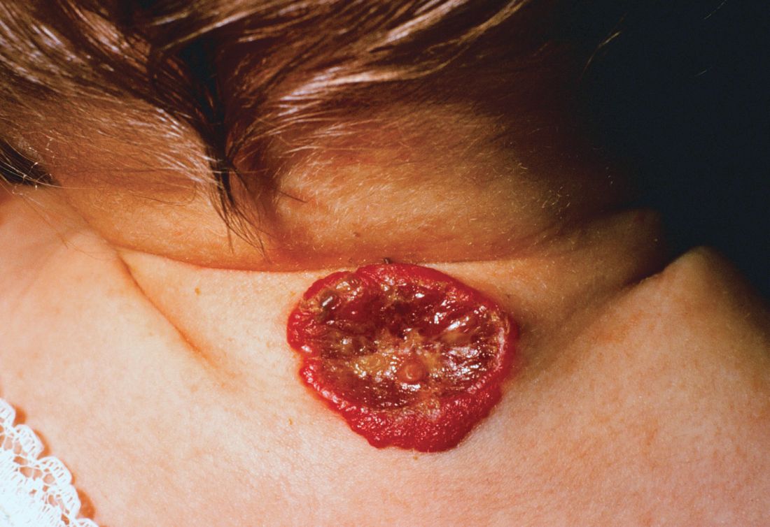
One clinical clue to picking up an infantile hemangioma (IH) that’s destined to ulcerate is an early grayish to white discoloration of the lesion, said Dr. Puttgen, chief of the division of pediatric dermatology at Johns Hopkins Medicine, Baltimore.
“Multimodal therapy is an absolute necessity” in treating an ulcerated IH, said Dr. Puttgen. Using an “all hands on deck” approach – a combination of topical and systemic modalities – can help bring the lesion under control.
Beta-blockers are first-line therapy to manage complicated IHs, with propranolol yielding a 98% response rate for all complicated IHs in the literature, said Dr. Puttgen.
Propranolol can decrease the volume and color of IHs and speed involution, in part by its ability to continue working after the proliferative growth phase of an IH. It’s also been shown to reduce the need for surgery in nasal IH, and it’s well tolerated, she added.
Evidence-based therapies for ulcerated hemangiomas include systemic propranolol at 1-3 mg/kg per day. That protocol will result in a healed ulcer within 2-6 weeks in most of the published case series, Dr. Puttgen noted.
Topical timolol also has evidence supporting its use for an ulcerated IH, and it has been found generally safe. In one study of 30 patients with IH, she said, three had mild adverse events consisting of sleep disturbance, diarrhea, and acrocyanosis. Another study reported success when brimonidine 0.2% and timolol 0.5% were used together. It’s possible, said Dr. Puttgen, that there’s a synergistic effect when combining the selective alpha-2 adrenergic agonist effect of brimonidine with timolol, which provides nonselective beta adrenergic blockade. However, she said, there has been an isolated report of brimonidine toxicity.
The ulcerated IHs need wound care, Dr. Puttgen added, with barrier creams and dressings. Pain management should be considered, because an ulcerated IH may have a large, friable, bleeding area. Pulsed-dye laser can also be a useful treatment modality for an ulcerating IH.
Going beyond the treatments for which the evidence is strongest and moving into more “state-of-the-art” treatments, “there may be a niche role for oral corticosteroids” as combination systemic therapy with propranolol, Dr. Puttgen said.
She shared images from a recently published report, in which she’s the senior author, showing the progression of an ulcerated IH. The hemangioma had received wound care and pulsed-dye laser treatment, and the infant was started on systemic propranolol. After 2 weeks, the IH had decreased significantly in volume, but the ulcerated area had actually increased. With the addition of oral corticosteroids, there was a reduction in ulceration after 2 weeks; and after 5 weeks of prednisolone, “the ulceration resolved without rebound,” said Dr. Puttgen. The corticosteroid was then tapered and propranolol was continued for an additional 2 months, then tapered. By 10 months, the IH had almost completely resolved (Br J Dermatol. 2017 Apr;176[4]:1064-7).
If a corticosteroid is added to propranolol, there may be benefit to a slower propranolol dose, Dr. Puttgen said. She suggests an altered dosing schedule, beginning with 1 mg/kg per day in two or three divided doses. Then, over a period of 2-7 days, the total daily dose can be increased to 1.5 mg/kg per day. Bumping the dose up to 2 mg/kg per day or higher should not happen until after 2 weeks at the reduced dosing schedule, she explained.
Dr. Puttgen disclosed that she is on the advisory board and has received honoraria from Pierre Fabre Dermatologie.
[email protected]
On Twitter @karioakes
EXPERT ANALYSIS FROM WCPD 2017

New-onset AF after aortic valve replacement did not affect long-term survival
New-onset atrial fibrillation after aortic valve replacement was not an independent risk factor for decreased long-term survival, according to the results of a single-center, retrospective study reported by Ben M. Swinkels, MD, of St Antonius Hospital, Nieuwegein, and his colleagues in the Netherlands.
Key to this success, however, is restoring normal sinus rhythm before hospital discharge, they said.
In this retrospective, longitudinal cohort study, 569 consecutive patients with no history of AF who underwent AVR with or without concomitant coronary artery bypass grafting during 1990-1993 were followed for a mean of 17.8 years (J Thorac Cardiovasc Surg. 2017;154:492-8).
Thirty-day and long-term survival rates were determined in the 241 patients (42%) with and the 328 patients (58%) without new-onset postoperative atrial fibrillation (POAF), which was defined as electrocardiographically documented AF lasting for at least several hours, and occurring after AVR while the patient was still admitted. Standard therapy to prevent new onset POAF was the use of sotalol in patients who were not on beta-blocker therapy, and continuation of beta-blocker therapy for those who were already on it.
There were no significant differences between the two groups in demographic characteristics. There were also no significant differences between the two groups in operative characteristics, postoperative in-hospital adverse events, and postoperative hospital lengths of stay until discharge home, except for mechanical ventilation time, which was significantly longer in the patients with new-onset POAF (P = .011).
Thirty-day mortality was 1.2% in the patients with POAF, and 2.7% in those without, a nonsignificant difference. There was no statistically significant difference between the two survival curves and the Kaplan-Meier overall cumulative survival rates at 15 years of follow-up in the patients with new-onset POAF vs. those without were not statistically different (41.5% vs. 41.3%, respectively).
In addition, the 18-year probability of long-term first adverse events, including recurrent AF, transient ischemic attack, ischemic or hemorrhagic stroke, peripheral venous thromboembolism, or major or minor bleeding was not significantly different between the two groups.
“New-onset POAF after AVR does not affect long-term survival when treatment is aimed to restore sinus rhythm before the patient is discharged home. Future studies with a prospective, randomized design should be done to confirm this finding in patients undergoing different kinds of cardiac surgery,” the researchers concluded.
The study was funded by the authors’ home institution; the authors reported they had nothing to disclose.
The incidence of atrial fibrillation after valve surgery has been described to be as high as 50%, Manuel J. Antunes, MD, said in an editorial commentary. “The adverse effect on long-term survival may not be related to the short-lived new-onset AF but rather to the underlying pathology associated to the arrhythmia, especially pathology that affects the myocardium, principally in atherosclerotic coronary artery disease,” he wrote. “It is not survival alone, however, that should be cause for concern; AF, even in episodes of limited duration, may result in transient ischemic attacks, ischemic, or hemorrhagic strokes, and peripheral thromboembolism, which is why affected patients should immediately be anticoagulated.”
This study, however, is at odds with previously published studies, with opposite conclusions, according to Dr. Antunes. Swinkels and his colleagues suggest that one of the reasons for the discrepancy was the homogeneous character of their series, which consisted almost entirely of patients who had isolated AVR. Dr. Antunes also adds that another important aspect to consider is that the antiarrhythmic drugs used prophylactically or therapeutically for this patient cohort (treated during 1990-1993) are no longer used or have been replaced by new and more efficacious pharmacologic agents.

Manuel J. Antunes, MD, of the University Hospital and Faculty of Medicine, Coimbra, Portugal, made these remarks in an invited editorial (J Thorac Cardiovasc Surg. 2017;154:490-1). He reported having nothing to disclose.
The incidence of atrial fibrillation after valve surgery has been described to be as high as 50%, Manuel J. Antunes, MD, said in an editorial commentary. “The adverse effect on long-term survival may not be related to the short-lived new-onset AF but rather to the underlying pathology associated to the arrhythmia, especially pathology that affects the myocardium, principally in atherosclerotic coronary artery disease,” he wrote. “It is not survival alone, however, that should be cause for concern; AF, even in episodes of limited duration, may result in transient ischemic attacks, ischemic, or hemorrhagic strokes, and peripheral thromboembolism, which is why affected patients should immediately be anticoagulated.”
This study, however, is at odds with previously published studies, with opposite conclusions, according to Dr. Antunes. Swinkels and his colleagues suggest that one of the reasons for the discrepancy was the homogeneous character of their series, which consisted almost entirely of patients who had isolated AVR. Dr. Antunes also adds that another important aspect to consider is that the antiarrhythmic drugs used prophylactically or therapeutically for this patient cohort (treated during 1990-1993) are no longer used or have been replaced by new and more efficacious pharmacologic agents.
Manuel J. Antunes, MD, of the University Hospital and Faculty of Medicine, Coimbra, Portugal, made these remarks in an invited editorial (J Thorac Cardiovasc Surg. 2017;154:490-1). He reported having nothing to disclose.
New-onset atrial fibrillation after aortic valve replacement was not an independent risk factor for decreased long-term survival, according to the results of a single-center, retrospective study reported by Ben M. Swinkels, MD, of St Antonius Hospital, Nieuwegein, and his colleagues in the Netherlands.
Key to this success, however, is restoring normal sinus rhythm before hospital discharge, they said.
In this retrospective, longitudinal cohort study, 569 consecutive patients with no history of AF who underwent AVR with or without concomitant coronary artery bypass grafting during 1990-1993 were followed for a mean of 17.8 years (J Thorac Cardiovasc Surg. 2017;154:492-8).
Thirty-day and long-term survival rates were determined in the 241 patients (42%) with and the 328 patients (58%) without new-onset postoperative atrial fibrillation (POAF), which was defined as electrocardiographically documented AF lasting for at least several hours, and occurring after AVR while the patient was still admitted. Standard therapy to prevent new onset POAF was the use of sotalol in patients who were not on beta-blocker therapy, and continuation of beta-blocker therapy for those who were already on it.
There were no significant differences between the two groups in demographic characteristics. There were also no significant differences between the two groups in operative characteristics, postoperative in-hospital adverse events, and postoperative hospital lengths of stay until discharge home, except for mechanical ventilation time, which was significantly longer in the patients with new-onset POAF (P = .011).
Thirty-day mortality was 1.2% in the patients with POAF, and 2.7% in those without, a nonsignificant difference. There was no statistically significant difference between the two survival curves and the Kaplan-Meier overall cumulative survival rates at 15 years of follow-up in the patients with new-onset POAF vs. those without were not statistically different (41.5% vs. 41.3%, respectively).
In addition, the 18-year probability of long-term first adverse events, including recurrent AF, transient ischemic attack, ischemic or hemorrhagic stroke, peripheral venous thromboembolism, or major or minor bleeding was not significantly different between the two groups.
“New-onset POAF after AVR does not affect long-term survival when treatment is aimed to restore sinus rhythm before the patient is discharged home. Future studies with a prospective, randomized design should be done to confirm this finding in patients undergoing different kinds of cardiac surgery,” the researchers concluded.
The study was funded by the authors’ home institution; the authors reported they had nothing to disclose.
FROM THE JOURNAL OF THORACIC AND CARDIOVASCULAR SURGERY
Key clinical point:
Major finding: Cumulative 15-year survival rates were similar in the patients with new-onset postop AF (41.5%) to those without (41.3%).
Data source: A retrospective longitudinal cohort study of 569 consecutive patients without a history of AF who were followed for a mean of 17.8 years after AVR with or without concomitant CABG.
Disclosures: The study was funded by the authors’ home institution and the authors reported they had nothing to disclose.

New test could cause OSA’s treatment success rate to rise
A novel device has shown a high rate of accuracy in predicting which patients with obstructive sleep apnea (OSA) will improve with oral appliance therapy, according to a study.
“At the present time CPAP is our go-to standard medical therapy [for treating OSA]. While it is a wonderful therapy, it has a very serious drawback, which is poor compliance, and that undercuts its long-term effectiveness in reducing the incidence of cardiovascular disease,” said John E. Remmers, MD, the principal investigator, in an interview.
Referring to the Sleep Apnea Cardiovascular Endpoints (SAVE) trial’s finding that continuous positive airway pressure (CPAP) did not reduce long-term cardiovascular incidents, he claimed that “these incidents are not being reduced by CPAP, because people don’t use it” (N Engl J Med. 2016 Sept 8;375[10]:919-31).
In Dr. Remmers’ new two-part study, 202 adults – primarily overweight, middle-aged men, diagnosed with moderate sleep apnea – were divided into two groups. The first included 149 people who were given a two-night, in-home, feedback controlled mandibular positioner (FCMP) test, using equipment manufactured by Zephyr Sleep Technologies. In this test, a custom-fit oral appliance is simulated using a temporary set of trays and impression material. The trays are connected to a small motor controlled by a little computer that sits on the stomach and moves the mandible when the patient has a problem breathing.
All patients received a custom oral appliance designed using data acquired from the test. The patients then wore the custom oral appliances while connected to a validated monitor as an outcomes study.
Finally, the researchers fed all of the data they collected from this first group of patients into a machine learning model. Then the second set of patients participated in the testing. Outcomes data on the appliance’s performance in each individual in the first group were used to create a classification system to predict therapeutic outcomes for the 53 patients in the second group. The patients in the second group then received their custom oral appliances, connected to the same type of monitor used by the first group.
Therapeutic success or failure was defined as having mean oxygen desaturation index values of less than or greater than 10 events/hour, respectively. The investigators determined that the test had an 85% sensitivity level with 93% specificity, a positive predictive value of 97%, and a negative predictive value of 72%. Of those who were predicted to respond to therapy, the mandibular protrusive position was efficacious in 86% of patients.
The high rate of accuracy for predicting who will derive the most benefit from the appliance, along with the demonstrated preference for oral appliances compared to continuous positive airway pressure devices among patients, increases the clinical utility of the appliance, and expands options for clinical management of sleep apnea, according to the study authors (Clin Sleep Med. 2017;13[7]:871-80).
“Our test allows the physician to prescribe the therapy knowing it will get rid of sleep apnea, and it tells the dentist how far the mandible needs to be pulled out by the custom fit device,” Dr. Remmers explained.
Dentists will also benefit from the test, because it allows them to make an appliance that will not need to be adjusted and will have a higher success rate than the current 60% success rate that oral appliances have at treating sleep apnea, he noted.
“This opens up a new an alternative clinical avenue at a critical time, when we have just learned over the past few years that there are serious questions about the effectiveness of CPAP in the long term,” Dr. Remmers added. “[With oral appliance therapy] you have an opportunity for higher compliance, because people prefer the less obtrusive oral appliance therapy over CPAP, and they use it more than CPAP. ... Because our product says you don’t treat everybody, you only undertake oral appliance therapy for those who we know in advance will have a favorable outcome, it removes a major barrier to oral appliance therapy that has been the barrier for many years.”
Dr. Remmers noted that his test was not nearly as good at identifying people who would be failures as it was at identifying people who would be successes and that he is carrying out another trial with a similar device.
Some participants reported sore gums when using the device, but there were no long-lasting adverse events reported.
The mandibular positioner home test has not been approved or cleared for use by the Food and Drug Administration, but is currently being sold in Canada, according to Dr. Remmers.
Zephyr Sleep Technologies and Alberta Innovates Technology Futures sponsored the study. It is registered on clinicaltrials.gov as NCT03011762. All of the investigators, other than Nikola Vranjes, are employed or associated with Zephyr Sleep Technologies.
Whitney McKnight contributed to this report.
Say ‘Aloha’ to the best health care
It probably should come as no surprise that Hawaii, which has been named the healthiest state for 5 consecutive years, is now being honored for having the best health care by personal finance website WalletHub.
The state’s high scores in two of the three broad dimensions of health care – first in outcomes and third in cost – used in the WalletHub analysis allowed it to overcome its ranking of 42nd in the third dimension, access, and finish ahead of Iowa and Minnesota, which tied for second. New Hampshire earned a fourth-place finish and the District of Columbia was fifth, courtesy of its first-place finish in the cost dimension, WalletHub reported. Maine, which finished 14th overall, was No. 1 in access.
The state in 51st place is Louisiana, which placed in the top 5 in both cancer and heart disease rates. Mississippi was credited with the 50th-best health care system, just behind Alaska (49), Arkansas (48), North Carolina (47), and Georgia (46). The lowest ranking in each dimension went to Alaska (cost), Texas (access), and Mississippi (outcomes), according to WalletHub’s analysts.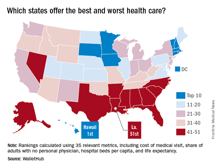
A closer look at some of the individual metrics shows that the District of Columbia has the most physicians per capita and Idaho has the fewest, Medicare acceptance is highest among physicians in North Dakota and lowest in Hawaii, and infant mortality is lowest in New Hampshire and highest in Mississippi, according to the WalletHub analysis, which was based on data from 19 sources, including the Centers for Medicare & Medicaid Services, the Association of American Medical Colleges, and the Social Science Research Council.
IV ketamine proves superior to active placebo in low, high doses
MIAMI – Intravenous ketamine in a range of doses is superior to active placebo, according to analyses from a study of the drug for treatment-resistant depression.
Most of the effect was attributable to differences recorded at Day 1 of the 3-day study, according to George I. Papakostas, MD, scientific director of the Massachusetts General Hospital Clinical Trials Network and Institute and coinvestigator of the study, who presented these findings at a meeting of the American Society of Clinical Psychopharmacology, formerly the New Clinical Drug Evaluation meeting.
The 99 adults with treatment-resistant depression – primarily white women in their mid-40s – were randomly assigned either to an active placebo group given 0.045 mg/kg of midazolam or to one of four treatment arms given a single infusion of intravenous ketamine at either 0.1 mg/kg, 0.2 mg/kg, 0.5 mg/kg, or 1.0 mg/kg.
Baseline scores on the 6-item Hamilton Depression Rating Scale (HAMD-6) ranged between 12.6 and 13.1 across the study.
To determine the efficacy of intravenous ketamine at different doses over the course of 72 hours, Dr. Papakostas, who also directs treatment-resistant depression studies at Massachusetts General, and his colleagues used multiple statistical models. The first analysis was a comparison of the effects of the active placebo and all ketamine groups combined at Day 1 and at Day 3.
At Day 1, the change in baseline HAMD-6 scores for all the ketamine arms combined, compared with the active placebo group, was statistically significant (P = .0278). At Day 3, the change in baseline HAMD-6 scores for the combined ketamine groups, compared with the active placebo arm, also was statistically significant (P = .0391).
A secondary analysis of the patient-reported Symptoms of Depression Questionnaire also showed a statistically significant improvement (P = .09) from baseline in the combined ketamine groups, compared with the active placebo group.
At Day 1, the combined ketamine groups’ changes from baseline HAMD-6 were –3.25 with an effect size of 0.86, a statistically significant finding. However, by the Day 3, the combined ketamine groups’ effects size fell away. “There is no longer a statistically significant difference, so it’s a rapid effect – like we’ve seen in the other studies for the combined doses – but it is not an effect that is sustained,” said Dr. Papakostas, also an associate professor of psychiatry at Harvard Medical School, Boston.
For the individual doses, compared with active placebo, the ketamine 0.1 mg/kg arm had an overall –0.35 change in baseline HAMD-6 scores, which Dr. Papakostas said had “a large effect size of 0.82.”
Dr. Papakostas also said the ketamine 0.2 mg/kg arm “did not really seem to move things around at all.” Meanwhile, the 0.5 mg/kg and 1.0 mg/kg arms each had “big differences” in baseline HAMD-6 scores, compared with active placebo, of –4.79 and –3.76, respectively. They also exhibited statistically significant effect sizes of 1.21 and 0.95 at Day 1, respectively. However, at Day 3, there were neither numerical nor statistical differences, indicating the effect is not sustained.
Changes in the Symptoms of Depression Questionnaire for the combined drug arms at Day 1 were statistically significant with an unadjusted P value of .07 and an adjusted P value of .13.
Results for the Clinician Administered Dissociative States Scale showed that neither the ketamine 0.1 mg/kg arm nor the ketamine 0.2 mg/kg arm separated from active placebo, while the ketamine 0.5 mg/kg arm and the ketamine 1.0 mg/kg arm were each different from active placebo to numerically and statistically significant degrees. Each of the 0.5 mg/kg and the 1.0 mg/kg ketamine arms were associated with rises in blood pressure, according to Dr. Papakostas.
“So, it seems as though the doses that caused a dissociation seemed to cause a clinical effect that is equivalent, whereas in the lower doses, there didn’t seem to be any dissociative effects or blood pressure effects,” Dr. Papakostas said. “If you combine the findings, in my opinion, there is a signal in the 0.1 mg/kg treatment arm, even though it just misses it on the P value.”
Dr. Papakostas said that, although more data are needed to determine optimal dosing and a clearer risk-benefit ratio, the results suggested that intravenous ketamine could offer transient, beneficial effects for patients with treatment-resistant depression.
Dr. Papakostas is the scientific director of the MGH Clinical Trials Network and Institute. This study’s coinvestigator, Maurizio Fava, MD, has numerous relevant financial ties to industry. This trial was part of the National Institute of Mental Health’s Rapidly-Acting Treatments for Treatment-Resistant Depression research program.
[email protected]
On Twitter @whitneymcknight
FROM THE ASCP ANNUAL MEETING
Key clinical point:
Major finding: Ketamine’s effect size and improvement from baseline depression scores showed significant separation from placebo in most analyses conducted in this study.
Data source: Multicenter, randomly controlled, double-blind study of 99 adults with treatment-resistant depression given active placebo or various doses of intravenous ketamine.
Disclosures: Dr. Papakostas is the scientific director of the Massachusetts General Hospital Clinical Trials Network and Institute. This study’s coinvestigator, Dr. Maurizio Fava, has numerous relevant financial ties to industry. This trial was part of the National Institute of Mental Health’s Rapidly-Acting Treatments for Treatment-Resistant Depression research program.
VIDEO: How to prevent, manage perinatal HIV infection
PARK CITY, UTAH – Despite notable progress in recent years, . Early recognition and treatment of HIV infection in pregnancy, prophylaxis for at-risk women, and retention of infected women in postpartum HIV care remain important goals, but they aren’t always met.
In a wide-ranging interview at the annual scientific meeting of the Infectious Diseases Society for Obstetrics and Gynecology, Gweneth Lazenby, MD, associate professor of obstetrics and gynecology at the Medical University of South Carolina, Charleston, explained what to do to improve the situation. Among the many pearls she shared: One HIV test isn’t enough for at-risk women.
AT IDSOG